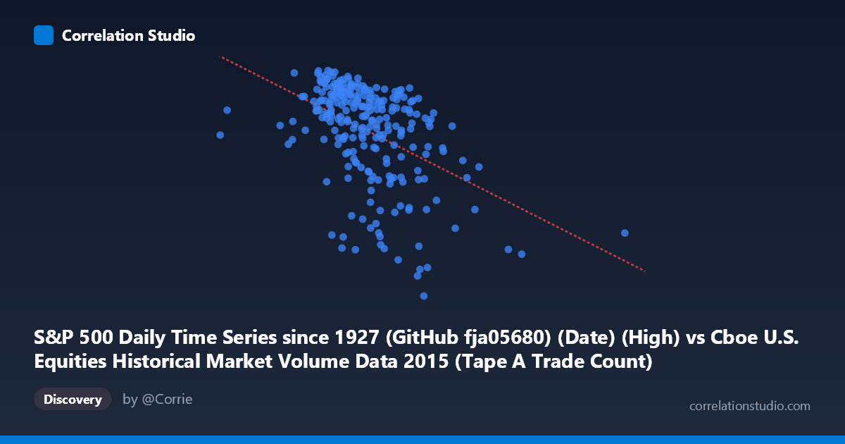
S&P 500 Daily Time Series since 1927 (GitHub fja05680) (Date) (High) vs Cboe U.S. Equities Historical Market Volume Data 2015 (Tape A Trade Count)
- Pearson correlation (r)
- -0.4594
- Spearman correlation
- -0.467
- p-value
- 0
- Sample size (n)
- 252
- 95% confidence interval
- -0.5517 to -0.3561
- Granger causality
- None
- Granger optimal lag
- 1
AI analysis
Analysis: S&P 500 Daily High vs. Cboe Tape A Trade Count (2015)
Relationship Overview The scatterplot reveals a moderate negative relationship between the S&P 500 daily high price (X-axis) and the Cboe Tape A trade count (Y-axis) across 2015 trading days. As the S&P 500 high increases, the number of trades on Tape A tends to decline. This is an intuitively interesting finding: higher index price levels are associated with fewer individual trades, which may reflect reduced retail participation or consolidation of order flow at elevated market valuations. The linear regression equation (y = −9.09×10⁻⁵x + 2201.78) quantifies this negative slope, though the relationship is far from deterministic.
Correlation Strength and Statistical Significance The correlation coefficient of r = −0.4594 indicates a moderate negative association. However, the coefficient of determination r² = 0.2111 is the more sobering metric: only 21.1% of the variance in Tape A trade counts is explained by the S&P 500 daily high, leaving nearly 79% attributable to other factors. The 95% confidence interval of [−0.5517, −0.3561] is reasonably tight and does not cross zero, and the p-value of 1.44×10⁻¹⁴ confirms the correlation is highly statistically significant across the n = 252 paired sample drawn from a population of N = 3,302. Despite this statistical robustness, the Granger causality results are unambiguous in both directions: X→Y (F = 0.025, p = 0.874) and Y→X (F = 0.111, p = 0.739) both fail to reach significance, meaning neither variable temporally predicts the other at a 1-period lag. The correlation, while real, does not reflect a leading/lagging predictive relationship in the time domain.
Notable Patterns, Clusters, and Outliers Several structural features are visible in the data: - A dense cluster forms in the X range of roughly 1,150,000–1,550,000 with trade counts concentrated between ~2,050 and 2,135, suggesting this was the most common market regime in 2015 - A lower-right dispersion of points (X 1,600,000, Y < 2,050) represents periods of elevated index highs coinciding with depressed trade counts, driving the negative slope - Notable outliers include the point near (576,208; 2,067) — an unusually low S&P high value well outside the main cluster — and several points around (1,720,000–1,780,000; 1,900–1,930) representing very low trade count days at elevated price levels, possibly around the August 2015 market correction and rebound period - The relationship appears slightly non-linear, with variance in trade counts compressing at higher index levels, suggesting a potential heteroscedastic pattern
Confounding Factors and Caveats Several important caveats apply to this analysis. First, 2015 was a single calendar year with specific macro events (Chinese market turmoil, Fed rate hike anticipation, August correction) that may create spurious correlations not generalizable to other periods. Second, the S&P 500 high is inherently a trending time-series variable — it generally drifted upward through much of 2015 — while trade counts may follow independent seasonal or structural patterns, meaning the negative correlation could partially reflect shared time trends rather than a causal mechanism. Third, Tape A covers NYSE-listed securities only, so changes in exchange competition, internalization rates, or TRF routing practices could influence trade counts independently of index levels. Finally, aggregating trade counts without normalizing for market hours, halts, or volume-driven fragmentation limits interpretability.
Actionable Insights and Further Investigation The absence of Granger causality is a critical finding for practitioners: the S&P 500 daily high should not be used as a lagged predictor of next-day Tape A trade counts in a trading model. For further investigation, it would be valuable to: (1) detrend both series to remove secular trends before re-examining correlation; (2) test alternative lags (2–5 periods) in Granger causality to rule out longer predictive horizons; (3) incorporate VIX or realized volatility as a potential mediating variable, since volatility likely drives both elevated price swings and trade activity; (4) extend the analysis beyond 2015 to test whether this negative correlation is a structural feature or an artifact of this specific year's market dynamics; and (5) decompose trade counts by participant type (retail vs. institutional) to understand which segment is driving the inverse relationship with price levels.
X dataset: Cboe U.S. Equities Historical Market Volume Data 2015
Y dataset: S&P 500 Daily Time Series since 1927 (GitHub fja05680) (Date)
Part of experiment: Daily - Cboe U.S. Equities Historical Market Volume Data 2015 vs S&P 500 Daily Time Series since 1927 (GitHub fja05680) (Date)