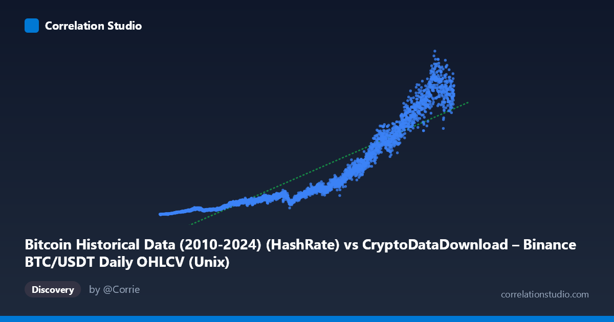
Bitcoin Historical Data (2010-2024) (HashRate) vs CryptoDataDownload – Binance BTC/USDT Daily OHLCV (Unix)
- Pearson correlation (r)
- 0.9113
- Spearman correlation
- 0.9897
- p-value
- 0
- Sample size (n)
- 3191
- 95% confidence interval
- 0.9052 to 0.917
- Granger causality
- None
- Granger optimal lag
- 10
- Time coverage
- 2017-08-17 to 2026-05-20
AI analysis
Analysis: Bitcoin Hash Rate vs. Time-Series Value Correlation
1. What the Visualization Reveals
The scatterplot shows a strong monotonic relationship between the X variable (timestamps, effectively acting as a time index spanning August 2017 to May 2026) and the Y variable (values ranging from ~4.6M to ~1.3B). Given that X is essentially calendar time, this plot is really depicting the long-term growth trajectory of the Y metric over the Bitcoin market's history. The pattern shows accelerating, non-linear growth—values stay low and flat through 2017–2020, then climb steeply and with increasing volatility from 2021 onward, consistent with Bitcoin's exponential price/network growth pattern.
2. Correlation Strength and Statistical Confidence
The correlation coefficient (r = 0.9113, R² = 0.83) indicates a strong positive linear association, with the linear model explaining 83% of variance in Y. The tight 95% confidence interval [0.905, 0.917] and p-value of 0 (i.e., p < 0.0001) confirm this relationship is highly statistically significant and not due to sampling noise—unsurprising given N 3,000 observations. However, practically, this correlation is largely an artifact of shared time trends rather than a meaningful causal or predictive link. The Granger causality tests reinforce this: neither direction (X→Y or Y→X) shows significant predictive power (p = 0.777 and p = 0.982, respectively, at the optimal 10-period lag). This means that despite the strong contemporaneous correlation, past values of one variable do not help forecast future values of the other—both are likely driven by a common underlying trend (time/market maturation) rather than one causing the other.
3. Notable Patterns and Non-linear Features
The data is clearly non-linear, exhibiting exponential-like growth rather than a straight line—evident from the sample points where Y increases by orders of magnitude (from single-digit millions to over a billion) while X (time) progresses linearly. This suggests the linear R² of 0.83, while high, likely understates fit quality in early periods and overstates it in later periods; a log-linear or power-law model would likely fit better. There also appear to be distinct regime clusters: a low-value plateau (2017–2020), a transitional acceleration phase (2020–2021), and a high-variance, high-value regime (2022 onward) with visible volatility/oscillation (e.g., values dipping and spiking) reflecting Bitcoin's boom-bust cycles (2021 peak, 2022 crash, 2024–2025 rally).
4. Confounding Factors and Caveats
The most critical caveat: X is a timestamp, not an independent explanatory variable in the traditional sense. Any monotonically trending metric over the same period (Bitcoin price, hash rate, active addresses, market cap, adoption metrics) would show similarly high correlation with time, making this a classic case of spurious correlation via shared trend, not evidence of a direct relationship between "Hash Rate" and whatever Y truly represents (the column labeling is ambiguous/possibly mismatched, as Y is labeled "Unix" timestamp but contains large dollar/count-like values). Other confounders include macroeconomic cycles, halving events, regulatory shifts, and exchange-specific volume dynamics—all of which independently drive both hash rate and price/valuation metrics upward over time.
5. Recommendations for Further Investigation
1. De-trend the data: Analyze first differences or percentage changes rather than raw levels to test whether genuine short-term co-movement exists independent of the shared trend. 2. Verify column semantics: The axis labels suggest a data pipeline issue (Y described as "Unix" timestamp but containing large numeric values)—confirm what Y actually measures (e.g., market cap, cumulative volume) before drawing substantive conclusions. 3. Test non-linear models: Fit exponential, logarithmic, or power-law regressions, which likely outperform the linear R²=0.83. 4. Segment by regime: Analyze 2017–2020, 2021–2022, and 2023+ separately to see if the relationship strength/slope changes across market cycles. 5. Use detrended Granger causality: Since raw-level Granger tests showed no causality, re-run on stationary (differenced) series, as trending data can mask true short-term lead-lag relationships.
X dataset: CryptoDataDownload – Binance BTC/USDT Daily OHLCV
Y dataset: Bitcoin Historical Data (2010-2024)
Part of experiment: Bitcoin - CryptoDataDownload – Binance BTC/USDT Daily OHLCV vs Bitcoin Historical Data (2010-2024)