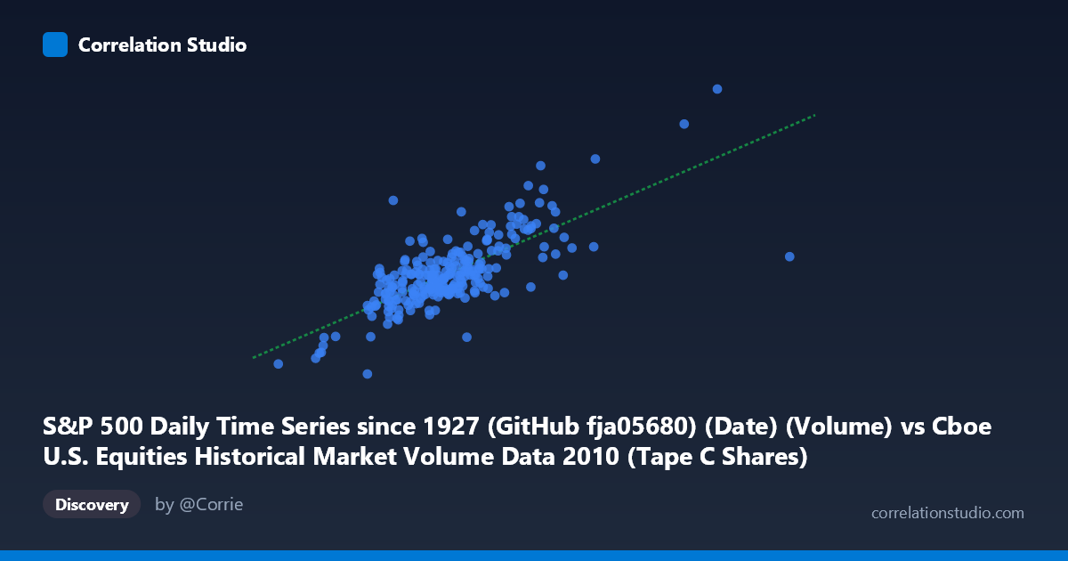
S&P 500 Daily Time Series since 1927 (GitHub fja05680) (Date) (Volume) vs Cboe U.S. Equities Historical Market Volume Data 2010 (Tape C Shares)
- Pearson correlation (r)
- 0.7453
- Spearman correlation
- 0.6795
- p-value
- 0
- Sample size (n)
- 252
- 95% confidence interval
- 0.6848 to 0.7956
- Granger causality
- None
- Granger optimal lag
- 10
AI analysis
Scatterplot Analysis: S&P 500 Daily Volume vs. Cboe Tape C Shares (2010)
Relationship Overview The scatterplot reveals a moderate-to-strong positive relationship between total U.S. equities market volume (X-axis, measured in shares traded across all exchanges and TRFs) and Cboe Tape C shares specifically. As aggregate daily market volume increases, Tape C share volume rises correspondingly, which is intuitive — Tape C covers NYSE Arca-listed securities, and its activity naturally scales with broader market participation. The linear regression equation (y = 18.70x + 1.39×10⁹) suggests that for every additional share of aggregate volume, Tape C volume increases by roughly 18.7 shares, with a substantial baseline intercept reflecting Tape C's persistent baseline trading activity even on lower-volume days.
Correlation Strength and Statistical Significance The Pearson correlation of r = 0.7453 indicates a meaningful positive association, and the R² of 0.5555 means approximately 55.5% of the day-to-day variance in Tape C volume is explained by aggregate market volume. While substantial, this also means nearly 45% of Tape C's variability is driven by other factors not captured here. The 95% confidence interval of [0.6848, 0.7956] is relatively tight given n = 252, reinforcing that the correlation estimate is stable and not an artifact of small-sample noise. The p-value of effectively zero confirms the relationship is highly statistically significant across the broader N = 3,302 population context. However, the Granger causality tests tell a notably different story: neither direction (X→Y: F = 1.02, p = 0.43; Y→X: F = 0.78, p = 0.65) achieves significance at the optimal 10-period lag. This means that while the two series are strongly contemporaneously correlated, neither series reliably predicts the other's future movements — they move together but do not lead or lag each other in a statistically meaningful way.
Notable Patterns, Clusters, and Outliers The data exhibits a broadly linear trend with a visible central cluster concentrated around X ≈ 130M–200M and Y ≈ 3.5B–5.5B, consistent with typical 2010 trading days. There are several notable high-leverage points in the upper-right region — particularly one observation near (349M, 9.47B) — that appear to be high-volume outlier days, potentially corresponding to macro events (e.g., Flash Crash aftermath, FOMC announcements, or index rebalancing days). On the lower end, one point near (109M, 1.29B) represents an unusually low Tape C reading relative to aggregate volume, suggesting potential data anomalies or a day when trading was heavily concentrated outside Tape C securities. The scatter also shows increased vertical spread at higher X values, hinting at mild heteroscedasticity — as overall volume grows, the variability in Tape C's share becomes less predictable.
Confounding Factors and Caveats Several important caveats apply. First, both variables are volume metrics from the same market ecosystem in the same year (2010), making contemporaneous correlation almost structurally inevitable — they share common drivers like market-wide risk appetite, volatility regimes (VIX spikes), and macroeconomic news flow. This shared latent driver likely inflates the observed correlation without implying a direct causal mechanism between the two series. Second, 2010 was a distinctive market year, marked by the May 6 Flash Crash and significant post-financial-crisis recovery dynamics, meaning patterns observed here may not generalize to other periods. Third, the linear regression assumes homoscedastic, normally distributed residuals — the visual evidence of spread widening at higher volumes suggests this assumption may be violated, potentially making confidence intervals slightly optimistic. Finally, the mismatch in dataset source labeling (X-axis label references S&P 500 data while Y-axis references Cboe data, and vice versa) warrants careful verification that the axis assignments reflect the intended variable mapping.
Actionable Insights and Further Investigation Practitioners interested in Tape C volume forecasting should recognize that aggregate market volume is a useful but incomplete predictor — R² ≈ 0.56 leaves substantial unexplained variance that may be recoverable through additional features. Suggested next steps include: (1) incorporating VIX or realized volatility as a covariate, since volatility spikes disproportionately affect volume across all tapes; (2) segmenting the analysis by day-of-week or month to detect seasonal patterns within 2010; (3) investigating the identified outlier days individually to determine whether they represent data quality issues or genuine market events worthy of regime-specific modeling; and (4) extending the analysis across multiple years to test whether the r ≈ 0.75 relationship is stable or drifts as market structure evolves (e.g., with changes in HFT activity or exchange competition). The absence of Granger causality also suggests that lagged volume signals alone are insufficient for predictive trading strategies and that contemporaneous, structural approaches would be more appropriate.
X dataset: Cboe U.S. Equities Historical Market Volume Data 2010
Y dataset: S&P 500 Daily Time Series since 1927 (GitHub fja05680) (Date)
Part of experiment: Daily - Cboe U.S. Equities Historical Market Volume Data 2010 vs S&P 500 Daily Time Series since 1927 (GitHub fja05680) (Date)