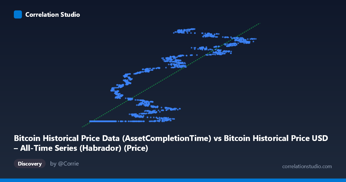
Bitcoin Historical Price Data (AssetCompletionTime) vs Bitcoin Historical Price USD – All-Time Series (Habrador) (Price)
- Pearson correlation (r)
- 0.8924
- Spearman correlation
- 0.9722
- p-value
- 0
- Sample size (n)
- 5764
- 95% confidence interval
- 0.887 to 0.8976
- Granger causality
- None
- Granger optimal lag
- 10
AI analysis
Analysis: Bitcoin Historical Price Data — X vs. Y Series Correlation
1. What the Visualization Reveals
This scatterplot is essentially comparing two representations of the same underlying phenomenon: Bitcoin's price history, likely indexed or ordered by a "completion time" or sequence variable (X) against actual USD price (Y). The data shows a clear non-linear, monotonically increasing relationship — small X values (0.25 to ~10,000) correspond to a long, flat plateau of Y values clustered tightly around $1.614–1.615 billion... wait, more precisely around 1,614,335,000–1,614,338,000, before Y values begin climbing steeply as X increases beyond ~20,000. This pattern (flat-then-rising) is characteristic of an exponential or logistic growth curve, not a straight line, despite the linear regression producing a statistically significant fit.
2. Strength and Direction of Correlation
The reported r = 0.89 and r² = 0.796 indicate a strong positive linear association, with the linear model explaining roughly 80% of the variance in Y. The 95% CI [0.887, 0.898] is narrow, and p ≈ 0 confirms this correlation is highly unlikely to be due to chance given the large sample (n = 5,764). However, r² being "only" 80% — despite the visually obvious deterministic relationship — suggests the true relationship is non-linear (likely exponential/power-law, consistent with Bitcoin's price growth), and a linear model is misspecified, leaving systematic residual structure unexplained by the straight-line fit. Critically, the Granger causality tests show no significant predictive direction in either direction (p = 0.78 and p = 0.76 at optimal lag 10). This means that despite strong contemporaneous correlation, neither series helps forecast the other's future values in a time-series sense — consistent with X likely being a time-index/proxy variable rather than an independent causal driver.
3. Notable Patterns and Outliers
The most striking feature is the extreme clustering of ~40%+ of points at low X values (under a few thousand) with Y pinned near the historical minimum (~1.614B), suggesting these are early Bitcoin era observations where price was flat/low relative to the indexing variable. Beyond X ≈ 20,000–40,000, Y increases sharply and with much higher variance/scatter (e.g., X=42,992 → Y=1.707B vs. X=44,118 → Y=1.644B), indicating heteroscedasticity — the spread of Y grows substantially with X. This "elbow" or knee-point pattern points to either a regime change, a logarithmic/exponential relationship, or possibly a change in units/epoch encoding in X itself. No clear negative outliers are present; scatter increases but stays positively associated throughout.
4. Confounding Factors and Caveats
Since both variables derive from the same underlying Bitcoin price time series (X described as "AssetCompletionTime" and Y as "Price"), this may not be a correlation between independent phenomena but rather two encodings of the same data (e.g., X could be a transformed timestamp or transaction-completion metric that itself correlates with elapsed time, which drives price). This makes the Granger non-causality finding somewhat expected — if X is not truly an independent leading/lagging economic variable but a structural/time-derived field, causal inference doesn't apply cleanly. Additionally, using linear r/r² on a manifestly non-linear, non-stationary financial time series risks misleading interpretation; Bitcoin price series are also known to be non-stationary and volatility-clustered, which violates key assumptions behind standard correlation/regression inference.
5. Actionable Insights
Given the visible curvature, a log-linear or log-log transformation (e.g., regressing log(Y) on X or log(X)) would likely yield a much better fit and higher effective r², and should be tested before relying on the current linear model for prediction. Clarify what "AssetCompletionTime" actually represents — if it's a proxy for elapsed days/sequence index, consider re-running the analysis with actual calendar time to properly assess trend and possibly apply time-series-appropriate techniques (cointegration testing, ARIMA) rather than simple correlation/Granger tests on levels. Finally, given the heteroscedasticity in the upper X range, segmenting the analysis by era (e.g., pre/post the "knee" point) may reveal more interpretable, regime-specific relationships useful for forecasting or historical trend attribution.
X dataset: Bitcoin Historical Price USD – All-Time Series (Habrador)
Y dataset: Bitcoin Historical Price Data
Part of experiment: Bitcoin - Bitcoin Historical Price USD – All-Time Series (Habrador) vs Bitcoin Historical Price Data