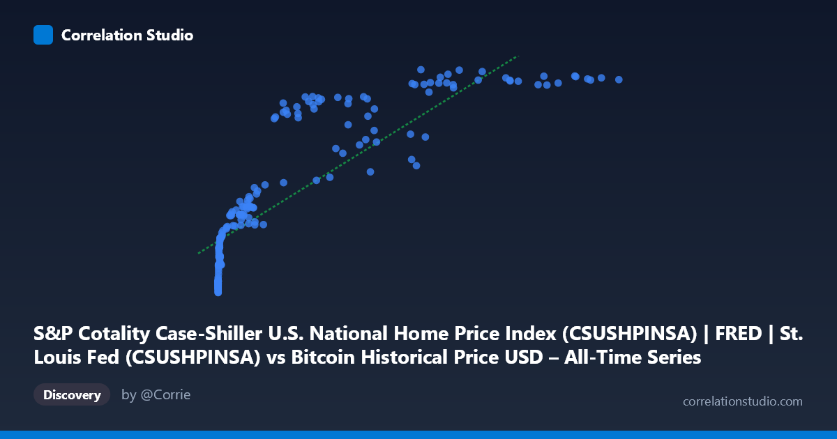
S&P Cotality Case-Shiller U.S. National Home Price Index (CSUSHPINSA) | FRED | St. Louis Fed (CSUSHPINSA) vs Bitcoin Historical Price USD – All-Time Series (Habrador) (Price)
- Pearson correlation (r)
- 0.8503
- Spearman correlation
- 0.9707
- p-value
- 0
- Sample size (n)
- 189
- 95% confidence interval
- 0.8053 to 0.8856
- Granger causality
- None
- Granger optimal lag
- 9
AI analysis
Analysis: Bitcoin Price vs. Case-Shiller Home Price Index
1. What the Visualization Reveals
The scatterplot shows a strong positive association between Bitcoin's historical USD price and the Case-Shiller U.S. National Home Price Index, but the relationship is clearly non-linear. At low Bitcoin values (under ~$1,000), home prices cluster tightly in the 135–190 range. As Bitcoin climbs into the tens of thousands, home prices rise more gradually and begin to plateau in the 290–330 range at the highest Bitcoin values (e.g., $85K–$118K). This produces a curved, logarithmic-like shape rather than a straight line — consistent with the note that Spearman's ρ exceeds Pearson's r.
2. Strength, Direction, and Uncertainty
With r = 0.848 and R² = 0.719, roughly 72% of the variance in home prices is statistically associated with Bitcoin price levels in this linear framing — a strong relationship by conventional standards. The 95% CI [0.802, 0.884] is tight and excludes zero, and the p-value of ~0 confirms this correlation is highly unlikely to be due to chance in this sample. However, correlation here almost certainly reflects shared time trends rather than a causal or mechanistic link. This is reinforced by the Granger causality tests: neither Bitcoin→Housing nor Housing→Bitcoin shows significant predictive power (p = 0.55 and p = 0.58 respectively). In other words, past values of one series do not help forecast future values of the other — the correlation is contemporaneous/trend-driven, not a leading/lagging causal relationship.
3. Notable Patterns and Outliers
- Compression at low X, expansion at mid X: Most of the dense low-value cluster (X < $2,000) corresponds to Bitcoin's early years (2010–2013), where home prices were still recovering from the 2008 crisis (~135–190). This creates a "hook" shape at the origin. - Ceiling effect at high X: Above ~$60K–$120K Bitcoin prices, home price index values compress into a narrow 315–331 band, suggesting the housing index is approaching a saturation/plateau relative to Bitcoin's continued volatility. - Local dips: Points like (56973, 278.51) and (45092, 244.17) and (58724, 249.78) sit noticeably below the general trend for their X-range, likely corresponding to Bitcoin bear-market crashes (2018, 2022) where BTC price fell sharply while home prices kept rising steadily — these are the clearest visual "outliers" breaking the monotonic pattern. - Log-like curvature: The overall shape suggests home prices scale with log(Bitcoin price) rather than linearly, which matches why a polynomial/log fit would outperform the linear R².
4. Confounding Factors and Caveats
The most important caveat: both series are trending time series over the same 2010–2026 window, and both have grown substantially over that period for entirely independent macroeconomic reasons (crypto adoption/speculation vs. housing supply, interest rates, and inflation). This is a classic case of spurious correlation via shared time trend — two unrelated variables that both increase over time will appear correlated even with no causal link, which the null Granger result strongly supports. Additionally, Bitcoin's extreme volatility (multiple 70-80% drawdowns) versus housing's comparatively smooth, monotonic climb means the relationship is asymmetric in variance and shouldn't be treated as a stable ratio.
5. Suggestions for Further Investigation
- De-trend both series (e.g., using year-over-year % changes or differencing) before correlating, to test whether the relationship survives once the shared upward trend is removed — this is critical to distinguish real co-movement from spurious trend correlation. - Fit a log-linear model (Y vs. log(X)) given the visual curvature and the Spearman/Pearson discrepancy; this will likely raise explained variance and better reflect the true functional form. - Segment by market regime (e.g., pre-2017, 2017–2021 crypto boom, 2022 crash, 2023+ recovery) to see if the correlation strength is stable or driven by a specific sub-period. - Treat this relationship as descriptive/associational only — it should not be used for predictive or trading purposes given the null Granger causality result and the strong likelihood of confounding via macro conditions (low interest rates, inflation, liquidity) that plausibly drove both asset classes upward independently.
X dataset: Bitcoin Historical Price USD – All-Time Series (Habrador)
Y dataset: S&P Cotality Case-Shiller U.S. National Home Price Index (CSUSHPINSA) | FRED | St. Louis Fed
Part of experiment: Bitcoin - Bitcoin Historical Price USD – All-Time Series (Habrador) vs S&P Cotality Case-Shiller U.S. National Home Price Index (CSUSHPINSA) | FRED | St. Louis Fed