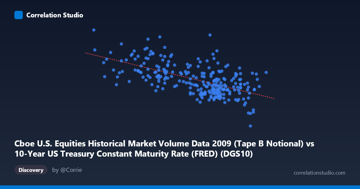
Cboe U.S. Equities Historical Market Volume Data 2009 (Tape B Notional) vs 10-Year US Treasury Constant Maturity Rate (FRED) (DGS10)
- Pearson correlation (r)
- -0.6046
- Spearman correlation
- -0.5768
- p-value
- 0
- Sample size (n)
- 250
- 95% confidence interval
- -0.6778 to -0.5195
- Granger causality
- None
- Granger optimal lag
- 10
AI analysis
Analysis of Cboe Tape B Notional Volume vs. 10-Year Treasury Yield (2009)
1. Overall Relationship The scatterplot reveals a moderate negative relationship between the 10-Year US Treasury Constant Maturity Rate (x-axis) and Cboe Tape B Notional trading volume (y-axis) across 2009. As Treasury yields rise, equity market notional volume tends to decline, and the linear regression equation (y = −2.03B·x + 11.92B) quantifies this: each one-percentage-point increase in the 10-year yield is associated with roughly a $2 trillion decrease in daily notional volume. Visually, the data cloud tilts downward from left to right, confirming the inverse association, though considerable scatter is evident throughout.
2. Correlation Strength, Direction, and Causality The Pearson correlation of r = −0.605 indicates a moderate-to-strong negative association, but the coefficient of determination r² = 0.366 clarifies that Treasury yields explain only about 36.5% of the variance in notional trading volume — leaving nearly two-thirds of variation unexplained by this relationship alone. The 95% confidence interval [−0.678, −0.520] is entirely negative and does not span zero, and the p-value of essentially 0 confirms the correlation is highly statistically significant in a sample of 250 paired observations drawn from a population of 3,232. However, Granger causality tests in both directions fail to reach significance (X→Y: F=1.59, p=0.111; Y→X: F=1.74, p=0.073), meaning neither variable demonstrably predicts the other temporally at any lag up to 10 periods. This is a critical caveat: the correlation is real and robust, but there is no evidence of a directional predictive (leading/lagging) relationship in the time series sense.
3. Notable Patterns, Clusters, and Outliers Several features stand out in the sample points. The yield range is fairly compressed (2.23–3.98%), yet volume spans nearly an order of magnitude (≈$1.3B to $9.5B), implying substantial day-to-day volume volatility independent of yield levels. There appear to be two loose clusters: a lower-yield cluster (x ≈ 2.3–3.0) with broadly higher and more dispersed volume, and a higher-yield cluster (x ≈ 3.4–3.9) with generally lower but still widely scattered volume. Notable outliers include the point near (3.82, 1.32B) — the lowest volume observation at a high yield — and several high-volume points at moderate yields, such as (2.78, 8.73B) and (2.95, 7.25B), which sit well above the regression line. The point (3.81, 4.12B) is less extreme but inconsistent with the cluster trend at high yields.
4. Confounding Factors and Caveats Several important caveats apply. First, 2009 was an exceptional year — the post-financial-crisis recovery, unprecedented Federal Reserve interventions (QE1 launched March 2009), and extreme market volatility all simultaneously drove both Treasury yields and equity trading volumes in ways that may not generalize. The negative correlation may partly reflect a risk-on/risk-off regime: when fear was high (low yields via flight to safety), equity trading volumes surged; as confidence returned (rising yields), volumes normalized. This is a classic omitted variable problem — investor risk sentiment is likely the common driver of both. Second, Tape B covers only a subset of equity exchanges (regional/non-primary), so volume patterns may differ from total market volume. Third, the daily granularity and relatively narrow yield range (1.75 percentage points) limit the generalizability of the linear model.
5. Actionable Insights and Further Investigation Given that over 63% of volume variance remains unexplained, several avenues merit investigation. Adding risk sentiment proxies — such as the VIX, credit spreads, or Fed announcement dates — as covariates in a multivariate model would likely substantially improve explanatory power and help isolate whether the Treasury-volume relationship survives controlling for market stress. Regime-segmentation analysis (pre- vs. post-QE1 in March 2009) could test whether the correlation is driven entirely by the crisis period. Researchers should also examine Tape A and C volume alongside Tape B to determine whether this pattern holds market-wide. Finally, while Granger causality was not detected at lags up to 10 periods, testing at shorter intraday frequencies or exploring nonlinear threshold models could reveal relationships obscured by the daily linear framework used here.
X dataset: 10-Year US Treasury Constant Maturity Rate (FRED)
Y dataset: Cboe U.S. Equities Historical Market Volume Data 2009
Part of experiment: Daily - 10-Year US Treasury Constant Maturity Rate (FRED) vs Cboe U.S. Equities Historical Market Volume Data 2009