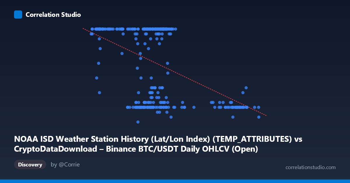
NOAA ISD Weather Station History (Lat/Lon Index) (TEMP_ATTRIBUTES) vs CryptoDataDownload – Binance BTC/USDT Daily OHLCV (Open)
- Pearson correlation (r)
- -0.4705
- Spearman correlation
- -0.3122
- p-value
- 0
- Sample size (n)
- 355
- 95% confidence interval
- -0.5478 to -0.3853
- Granger causality
- None
- Granger optimal lag
- 1
- Time coverage
- 2024-01-01 to 2024-12-31
AI analysis
Analysis of the Scatterplot Relationship
1. What the visualization reveals
The scatterplot shows a moderate negative relationship between the two variables, with a distinct clustering pattern rather than a smooth linear trend. Most data points concentrate in the X range of roughly 55,000–70,000, where Y values split into two dominant bands: a large cluster at Y=24 (the apparent ceiling of the scale) and a smaller cluster at low values (Y=7–12). A separate group of points at higher X values (90,000–100,000) consistently shows low Y values (8–11). This bimodal clustering suggests the relationship may be driven more by discrete regime shifts than by continuous covariation.
2. Strength, direction, and statistical confidence
The correlation coefficient (r = -0.4705) indicates a moderate negative association, with r² = 0.2214 meaning only about 22% of the variance in Y is explained by X — the majority (78%) is driven by other factors. The 95% CI [-0.5478, -0.3853] is reasonably tight and excludes zero, and the p-value of 0 confirms this relationship is highly unlikely to be due to chance given the large sample (n=355). However, statistical significance here reflects sample size more than practical strength — this is a weak-to-moderate relationship, not a tight predictive one. Critically, the Granger causality tests show no significant predictive direction in either direction (X→Y: p=0.71; Y→X: p=0.26), meaning that despite the contemporaneous correlation, neither variable helps forecast the other's future values based on past observations. This strongly suggests the correlation is either coincidental, driven by a shared external factor, or reflects a static/structural relationship rather than a dynamic causal one.
3. Notable patterns and outliers
The most striking feature is the ceiling effect at Y=24, which accounts for a large share of points across a wide X range (42,000–73,000). This suggests Y may be capped or censored at this value, artificially compressing variance and potentially inflating the apparent negative slope (since higher X points, clustered at 90,000+, all fall below this ceiling). Additionally, there are near-duplicate X values with wildly different Y outcomes (e.g., X≈65,300 giving both Y=24 and Y=9; X≈62,000–63,000 spanning Y=8 to Y=24), indicating high local variance and a weak instantaneous relationship at any fixed X. The high-X cluster (90,000–100,000) behaves almost like a separate regime with uniformly low Y, hinting at a threshold or non-linear effect rather than a continuous linear decline.
4. Confounding factors and caveats
Given the data provenance — one variable drawn from BTC/USDT OHLCV data and the other from NOAA weather station records — this pairing is almost certainly spurious or an artifact of mismatched/misaligned dataset joining (e.g., joined by row index or date rather than genuine domain linkage). Bitcoin prices and daily temperature/weather attributes have no plausible causal mechanism connecting them. The apparent correlation likely reflects coincidental trends over the 2024 time window (e.g., both series may have autocorrelated or seasonal patterns that happen to move in opposite directions over the year) rather than any real relationship. The ceiling effect at Y=24 further distorts the correlation estimate and violates linear regression assumptions (homoscedasticity, normality of residuals).
5. Actionable recommendations
Before drawing any substantive conclusions, verify the data-joining methodology — confirm that X and Y values are correctly paired by matching timestamps/dates rather than arbitrary row alignment. Investigate whether Y is genuinely capped at 24 (e.g., hours in a day, a categorical/ordinal encoding) and consider treating it as censored or ordinal data rather than continuous. Given the lack of Granger causality, this relationship should not be used for forecasting one variable from the other. If a real relationship is suspected, consider a controlled analysis with proper date alignment, seasonal decomposition, and testing for a shared confounding time trend (e.g., both series regressed against day-of-year) rather than relying on the raw cross-sectional correlation.
X dataset: CryptoDataDownload – Binance BTC/USDT Daily OHLCV
Y dataset: NOAA ISD Weather Station History (Lat/Lon Index)
Part of experiment: Bitcoin - CryptoDataDownload – Binance BTC/USDT Daily OHLCV vs NOAA ISD Weather Station History (Lat/Lon Index)