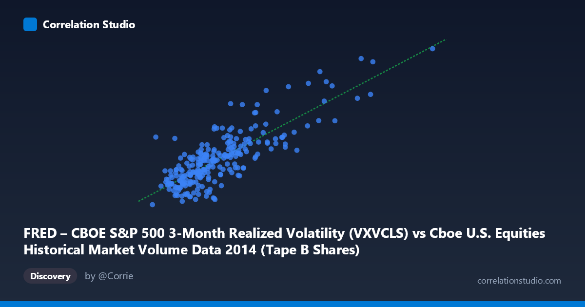
FRED – CBOE S&P 500 3-Month Realized Volatility (VXVCLS) vs Cboe U.S. Equities Historical Market Volume Data 2014 (Tape B Shares)
- Pearson correlation (r)
- 0.8168
- Spearman correlation
- 0.7521
- p-value
- 0
- Sample size (n)
- 252
- 95% confidence interval
- 0.7711 to 0.8542
- Granger causality
- None
- Granger optimal lag
- 1
AI analysis
Scatterplot Analysis: CBOE S&P 500 3-Month Realized Volatility vs. Tape B Shares Volume (2014)
Relationship Overview
The scatterplot reveals a moderately strong positive relationship between CBOE S&P 500 3-Month Realized Volatility (VXVCLS) on the X-axis and Tape B Shares trading volume on the Y-axis across 252 trading days in 2014. As realized volatility increases, Tape B share volume tends to rise in tandem, consistent with the well-established market microstructure principle that elevated uncertainty drives heightened trading activity. The linear regression equation (y = 6.95e-08x + 10.37) suggests that for every ~14.4 million unit increase in volume, volatility rises by approximately 1 point — though the causal direction of this relationship requires careful interpretation given the Granger results discussed below.
Correlation Strength and Statistical Significance
The Pearson correlation of r = 0.8168 is statistically robust, with an R² of 0.6672, meaning roughly 66.7% of the variance in volatility is explained by Tape B share volume — a substantively meaningful proportion for financial market data. The 95% confidence interval of [0.7711, 0.8542] is notably tight, reflecting the reasonable sample size (n = 252), and the p-value of ~0 confirms the relationship is highly unlikely to be a statistical artifact. However, the Granger causality results are strikingly null: neither direction (X→Y: F = 1.25, p = 0.26; Y→X: F = 0.0004, p = 0.98) achieves significance at any conventional threshold. This means that while the contemporaneous correlation is strong, neither variable's past values predict the other's future values — the two series move together but do not temporally lead or lag one another in a predictive sense.
Notable Patterns, Clusters, and Outliers
The sample points reveal a broadly linear trend punctuated by a distinct cluster of high-leverage outliers in the upper-right region, particularly observations near (155–162 million, 22–23 volatility), which correspond to identifiable stress episodes in late 2014 (likely October's sharp market selloff). The bulk of observations cluster tightly in the lower-left quadrant (~40–90 million volume, 12–18 volatility), suggesting the relationship is relatively stable during calm periods but stretches dramatically during market dislocations. There is also visible heteroscedasticity: variance in Y appears to fan outward as X increases, implying the linear model may underfit the high-volatility regime. One anomalous point near (51 million, 17.2) appears to defy the trend — high volatility with comparatively low volume — which may reflect a holiday-shortened or options-expiration day.
Confounding Factors and Caveats
Several important caveats apply. First, Tape B represents only a subset of U.S. equity volume (NYSE American and regional exchanges), so the correlation may partially reflect structural routing patterns rather than pure volatility-driven activity. Second, 2014 is a single calendar year with a specific macro backdrop (gradual Fed tapering, geopolitical shocks), limiting generalizability. Third, the absence of Granger causality suggests the relationship may be driven by a common latent factor — such as macro news arrival, institutional rebalancing cycles, or VIX-related hedging flows — rather than a direct volume-volatility mechanism. The heteroscedasticity also means the linear R² likely overstates model reliability in high-volatility regimes while understating it in calm periods.
Actionable Insights and Further Investigation
Practitioners and researchers should explore several follow-on analyses. First, fitting a log-linear or piecewise regression would better capture the apparent non-linearity at high-volatility extremes. Second, including additional volume tapes (A and C) alongside VIX (short-term) would allow decomposition of whether this effect is Tape B-specific or market-wide. Third, testing the relationship across multiple years (particularly 2008–2009 and 2020) would establish whether the 2014 coefficient is structurally stable or regime-dependent. Finally, incorporating intraday data and news event flags could help identify whether the contemporaneous co-movement is truly simultaneous or merely appears so at daily resolution — which would have direct implications for volatility-targeting strategies that rely on volume signals.
X dataset: Cboe U.S. Equities Historical Market Volume Data 2014
Y dataset: FRED – CBOE S&P 500 3-Month Realized Volatility
Part of experiment: Daily - Cboe U.S. Equities Historical Market Volume Data 2014 vs FRED – CBOE S&P 500 3-Month Realized Volatility