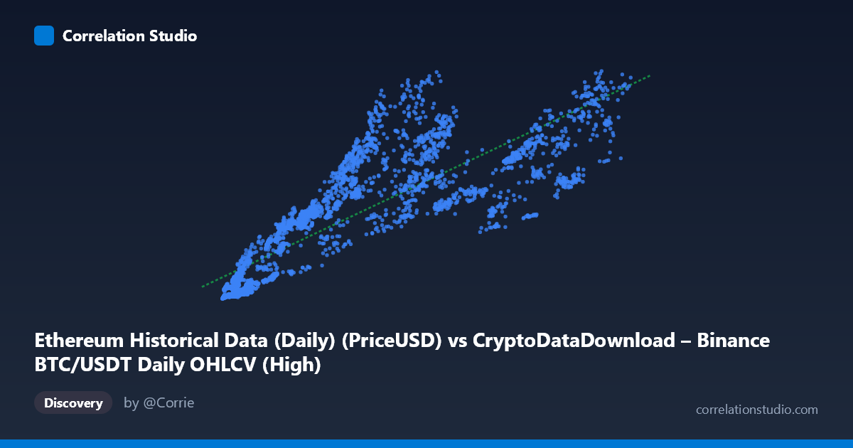
Ethereum Historical Data (Daily) (PriceUSD) vs CryptoDataDownload – Binance BTC/USDT Daily OHLCV (High)
- Pearson correlation (r)
- 0.8417
- Spearman correlation
- 0.9084
- p-value
- 0
- Sample size (n)
- 3191
- 95% confidence interval
- 0.8313 to 0.8515
- Granger causality
- None
- Granger optimal lag
- 4
- Time coverage
- 2017-08-17 to 2026-05-20
AI analysis
Scatterplot Analysis: BTC Price vs. ETH Price Metric
1. Relationship Overview
The scatterplot depicts a clear positive association between the BTC/USDT price series (X-axis) and what is labeled as an Ethereum-related price metric (Y-axis). Despite the mismatched column labels in the metadata (the X-axis description reference an ETH data column, while the header names suggest BTC pricing), the underlying pattern is consistent with two crypto assets that move together over time — as X increases from roughly $3,300 to $126,000, Y rises from under $100 to nearly $4,800. The relationship is broadly linear, though the scatter widens noticeably at higher X values, suggesting the linear model is a reasonable but imperfect fit.
2. Strength, Direction, and Statistical Confidence
The Pearson correlation of r = 0.84 indicates a strong positive linear relationship, and r² = 0.71 tells us that about 71% of the variance in Y can be statistically explained by X's linear trend — leaving roughly 29% of Y's variability attributable to other factors, noise, or non-linear dynamics. The tight 95% confidence interval [0.831, 0.852] combined with a p-value effectively at 0 confirms this correlation is highly statistically robust and not a product of sampling variability, especially given the large sample size (n=3,191). However, Granger causality testing reveals no significant predictive direction in either direction (X→Y: p=0.359; Y→X: p=0.541). This is a critical distinction: strong contemporaneous correlation does not imply that past values of one asset help forecast future values of the other. Practically, this suggests both series may be driven by a shared external factor (e.g., overall crypto market sentiment, macro liquidity conditions) rather than one asset leading the other temporally.
3. Notable Patterns and Outliers
Several features stand out in the sample data: - Heteroscedasticity: Variance in Y increases substantially as X grows — at low X (~$4,000–10,000), Y values cluster tightly between 130–450; at high X (~$80,000–110,000), Y ranges widely from ~1,565 to 4,277. This "fanning out" pattern violates the constant-variance assumption of simple linear regression. - Possible regime clusters: Data points seem to fall into distinct bands (e.g., low-price/low-Y cluster below X=15,000, a middle cluster from X=20,000–70,000, and a high-price cluster above X=80,000), possibly reflecting different market cycles or years within the 2017–2026 time span. - Mild outliers: Points like (84,300 → 1,565.57) and (84,720 → 1,813.00) sit below the general trend for that X range, while (62,420 → 3,392.70) sits above — indicating some decoupling during specific periods, possibly market-specific shocks (e.g., ETH-specific news vs. BTC-specific news).
4. Confounding Factors and Caveats
This correlation should be interpreted cautiously for several reasons: - Metadata inconsistency: The dataset descriptions are contradictory/mismatched (X-axis described as ETH PriceUSD but titled with a BTC dataset name; Y-axis described as BTC High but titled "Ethereum"). This ambiguity makes it hard to confirm which asset is truly which, and analysis should be revisited once labels are clarified. - Non-stationarity: Both time series (2017–2026) likely contain trends, structural breaks, and volatility clustering typical of crypto markets. Simple correlation on non-stationary series can be spurious or inflated — a common issue with two assets that both trended upward over multiple bull/bear cycles. - Shared macro drivers: BTC and ETH prices are both heavily influenced by common factors — overall crypto market sentiment, USD liquidity/interest rates, regulatory news, and exchange flows — which likely explains the strong correlation without direct causal linkage between the two specific series. - Time-aggregation issues: Daily OHLCV data can embed autocorrelation that inflates apparent correlation strength beyond what independent observations would show.
5. Actionable Insights and Next Steps
1. Clarify data provenance — resolve the labeling conflict between X and Y datasets before drawing further conclusions; verify with raw source files. 2. Test for cointegration rather than relying on simple correlation, since both series are likely non-stationary price levels — an Engle-Granger or Johansen test would clarify if there's a stable long-run equilibrium relationship despite the lack of Granger causality. 3. Analyze returns instead of price levels — converting to daily log returns would reduce spurious correlation from shared trends and better reveal genuine short-term co-movement or lead-lag relationships. 4. Segment by time period — given the wide time span (2017–2026) covering multiple bull/bear cycles, a rolling correlation analysis would reveal whether the relationship strengthens/weakens during specific market regimes (e.g., 2021 bull run vs. 2022 bear market). 5. Investigate the heteroscedasticity — consider a log-log transformation of both variables, which often stabilizes variance in financial price data and may improve model fit and interpretability of the regression coefficient.
X dataset: CryptoDataDownload – Binance BTC/USDT Daily OHLCV
Y dataset: Ethereum Historical Data (Daily)
Part of experiment: Bitcoin - CryptoDataDownload – Binance BTC/USDT Daily OHLCV vs Ethereum Historical Data (Daily)