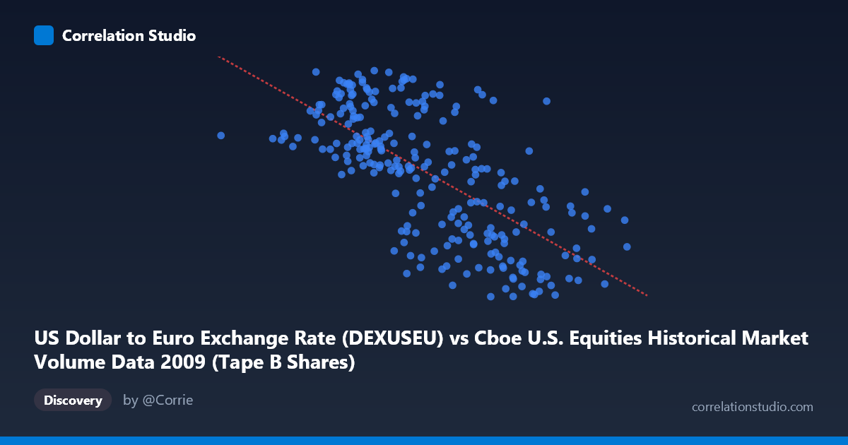
US Dollar to Euro Exchange Rate (DEXUSEU) vs Cboe U.S. Equities Historical Market Volume Data 2009 (Tape B Shares)
- Pearson correlation (r)
- -0.6798
- Spearman correlation
- -0.692
- p-value
- 0
- Sample size (n)
- 250
- 95% confidence interval
- -0.7414 to -0.607
- Granger causality
- None
- Granger optimal lag
- 1
AI analysis
Scatterplot Analysis: USD/EUR Exchange Rate vs. Cboe Tape B Share Volume (2009)
Relationship Overview The scatterplot reveals a moderate negative linear relationship between the US Dollar to Euro exchange rate and Cboe Tape B share volumes during 2009. As the exchange rate increases (a stronger dollar relative to the euro), Tape B share volumes tend to decrease, and vice versa. The linear regression equation (y = -1.15369E-09x + 1.56374) confirms this inverse relationship, with the steep negative coefficient indicating that each unit increase in volume corresponds to a meaningful decline in the exchange rate. The data points form a recognizable downward-sloping cloud, though with considerable scatter around the regression line, suggesting the relationship is real but far from deterministic.
Correlation Strength and Statistical Significance With r = -0.6798, this is a moderately strong negative correlation. The r² value of 0.4622 means that approximately 46.2% of the variance in the exchange rate is statistically explained by Tape B share volume — a substantial but incomplete explanatory share, leaving over half the variance attributable to other factors. The 95% confidence interval of [-0.7414, -0.6070] is relatively narrow and lies entirely in negative territory, reinforcing confidence that the inverse relationship is genuine rather than a sampling artifact. The p-value of essentially zero, combined with an N of 3,232, makes this correlation highly statistically significant. However, the Granger causality results are notably absent in both directions — neither X→Y (F = 0.0414, p = 0.8390) nor Y→X (F = 1.8948, p = 0.1699) shows predictive temporal power — meaning that while the two variables are correlated contemporaneously, neither reliably predicts the other's future values. This is a critical distinction: correlation without Granger causality suggests a shared common driver rather than any direct mechanistic link between these specific variables.
Notable Patterns and Outliers Several features stand out in the data distribution. The bulk of observations cluster between approximately 100M–200M on the X-axis and 1.30–1.50 on the Y-axis, forming a reasonably coherent central mass. At the lower end of the X-axis, including the notable point near 33.8M (the minimum), the exchange rate sits around 1.44, which aligns with the regression line but represents a sparse region. At the upper extreme (values approaching 243M–255M), exchange rates drop toward 1.26–1.27, consistent with the negative trend. A handful of points at moderate X-values show relatively high Y-values (e.g., ~111M paired with 1.50, ~133M with 1.50), suggesting upward outliers from the trend. The vertical spread within narrow X-bands is notable — for instance, near X ≈ 160–170M, Y-values range from roughly 1.28 to 1.49 — indicating substantial residual variance not captured by the linear model.
Confounding Factors and Interpretive Caveats The 2009 timeframe is highly context-specific: this was a period of extreme financial market volatility following the 2008 global financial crisis, with equity volumes elevated due to panic selling, institutional rebalancing, and high-frequency trading activity, while the USD/EUR rate was simultaneously influenced by Federal Reserve policy, ECB responses, and macroeconomic uncertainty. Both variables were likely driven by common macro shocks — risk-off episodes, for example, simultaneously spiked equity volumes and strengthened the dollar — which would generate observed correlation without any direct causal pathway. Additionally, the axis labels appear swapped in the dataset metadata (the X-axis column references exchange rate data while being labeled as market volume data, and vice versa), which warrants verification before drawing firm conclusions. Seasonality and day-of-week effects in equity trading could also introduce spurious structure, and the use of daily data means autocorrelation within each series may inflate apparent correlation strength.
Actionable Insights and Further Investigation Given the absence of Granger causality, practitioners should avoid using Tape B volume as a leading indicator for EUR/USD forecasting (or vice versa) in any trading or hedging strategy. Instead, the correlation likely reflects a latent common factor — such as aggregate market risk sentiment (e.g., the VIX), which should be incorporated as a control variable in any regression model. Recommended next steps include: (1) introducing risk sentiment proxies (VIX, credit spreads) to test whether they mediate or eliminate the observed correlation; (2) extending the analysis beyond 2009 to determine whether this relationship is structurally persistent or crisis-specific; (3) performing rolling-window correlation analysis to detect whether the relationship strengthens during high-volatility regimes; and (4) verifying the dataset column assignments to ensure X and Y variables are correctly mapped, given the apparent metadata inconsistency noted above.
X dataset: Cboe U.S. Equities Historical Market Volume Data 2009
Y dataset: US Dollar to Euro Exchange Rate
Part of experiment: Daily - Cboe U.S. Equities Historical Market Volume Data 2009 vs US Dollar to Euro Exchange Rate