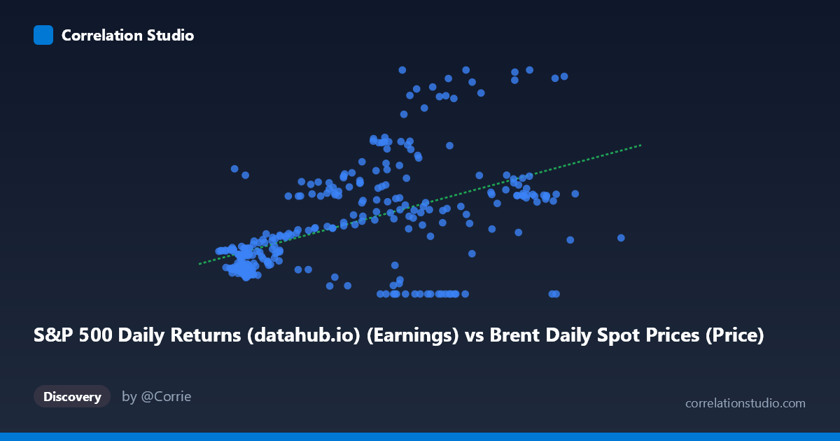
S&P 500 Daily Returns (datahub.io) (Earnings) vs Brent Daily Spot Prices (Price)
- Pearson correlation (r)
- 0.5158
- Spearman correlation
- 0.4874
- p-value
- 0
- Sample size (n)
- 297
- 95% confidence interval
- 0.4271 to 0.5947
- Granger causality
- None
- Granger optimal lag
- 1
AI analysis
Analysis: S&P 500 Earnings vs. Brent Crude Oil Prices
Relationship Overview The scatterplot reveals a moderate positive relationship between S&P 500 earnings (X-axis) and Brent crude oil spot prices (Y-axis) spanning nearly four decades (1987–2026). The linear regression equation y = 0.730x + 24.01 suggests that for every unit increase in S&P 500 earnings, Brent crude prices rise by approximately $0.73/barrel. While the upward trend is discernible, the substantial scatter around the regression line immediately signals that this relationship is far from deterministic, with many data points deviating dramatically from the fitted line — particularly at higher earnings values where vertical dispersion becomes pronounced.
Correlation Strength and Statistical Significance The Pearson correlation of r = 0.516 indicates a moderate positive association, but the more practically informative statistic is r² = 0.266, meaning S&P 500 earnings explain only 26.6% of the variance in Brent crude prices — leaving roughly 73.4% unexplained by this relationship alone. The 95% confidence interval [0.427, 0.595] is reasonably tight given N = 1,865, and the p-value of effectively zero confirms this correlation is statistically robust and not a sampling artifact. However, statistical significance should not be confused with practical or causal significance. Crucially, the Granger causality tests fail in both directions (X→Y: F = 1.40, p = 0.237; Y→X: F = 0.56, p = 0.457), meaning neither variable meaningfully predicts the other temporally at a 1-period lag. This strongly undermines any narrative of direct causal linkage, even though both series trend together over time.
Notable Patterns, Clusters, and Outliers Several structural features stand out in the data. A dense cluster of low-earnings, low-price observations (X < 30, Y < 50) dominates the lower-left region, likely corresponding to the pre-2000 era when both S&P earnings and oil prices were comparatively subdued. At higher earnings values (X 70), extreme vertical dispersion is striking — for example, points near X ≈ 85 span Y values from near 0 to approximately 190, which is nearly the full range of the dataset. Multiple Y ≈ 0 outliers appear at moderate-to-high X values (e.g., X = 67, 73, 85, 87), which likely represent data alignment anomalies, missing values coded as zero, or genuine oil price crashes (e.g., 2020 COVID collapse). These zero-value points are analytically problematic and may be artificially compressing the correlation estimate.
Confounding Factors and Caveats This correlation almost certainly reflects shared exposure to macroeconomic cycles rather than any direct causal mechanism between corporate earnings and oil prices. Both variables are heavily influenced by global GDP growth, inflation regimes, monetary policy cycles, and geopolitical events — meaning the observed r = 0.516 is likely a spurious correlation driven by common secular trends over the 1987–2026 period. The monthly sampling of S&P data paired with daily oil prices introduces temporal mismatch, which could systematically distort correlation estimates. Additionally, the Y ≈ 0 data points warrant immediate investigation, as including erroneous zeros would suppress the true correlation. The long time horizon also means the relationship may be structurally non-stationary — behaving very differently across distinct economic regimes (e.g., the 1990s, the commodity supercycle of 2002–2014, and the post-COVID era).
Actionable Insights and Further Investigation Given the failed Granger causality tests and modest r², practitioners should avoid using either variable as a direct predictor of the other in modeling frameworks. Instead, several follow-up analyses are recommended: (1) Remove or investigate zero-value Y observations before drawing any further conclusions; (2) Detrend both series (e.g., using first differences or percent changes) to test whether the correlation survives after removing shared long-run trends — this would reveal whether the relationship is substantive or purely trend-driven; (3) Segment analysis by economic regime (pre-2000, 2000–2014, 2014–present) to detect structural breaks; (4) Introduce intermediary variables such as global industrial production or USD index to test whether the correlation disappears under controls; and (5) explore non-linear specifications given the obvious heteroscedasticity at high earnings values, where a log-log or segmented regression might better characterize the relationship across different economic environments.
X dataset: Brent Daily Spot Prices
Y dataset: S&P 500 Daily Returns (datahub.io)
Part of experiment: Daily - Brent Daily Spot Prices vs S&P 500 Daily Returns (datahub.io)