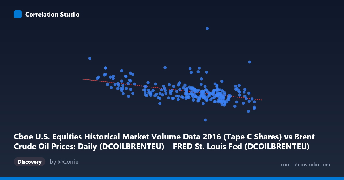
Cboe U.S. Equities Historical Market Volume Data 2016 (Tape C Shares) vs Brent Crude Oil Prices: Daily (DCOILBRENTEU) – FRED St. Louis Fed (DCOILBRENTEU)
- Pearson correlation (r)
- -0.4706
- Spearman correlation
- -0.4989
- p-value
- 0
- Sample size (n)
- 251
- 95% confidence interval
- -0.5617 to -0.3683
- Granger causality
- None
- Granger optimal lag
- 10
AI analysis
Analysis: Brent Crude Oil Prices vs. Cboe U.S. Equities Market Volume (2016)
Relationship Overview
The scatterplot reveals a negative relationship between Brent Crude Oil daily spot prices (X-axis) and Cboe U.S. equities market volume (Y-axis) across 251 trading days in 2016. The linear regression equation (y = -1,913,290x + 216,692,000) quantifies this inverse association: as oil prices rise, equity trading volume tends to decline. This pattern is visually consistent with several notable sample points — for instance, when X is near its lower bound (~26–32), Y values cluster at notably elevated levels (175M–229M shares), while at higher X values (~48–54), Y values compress into a tighter, lower range (~94M–165M). The relationship, while statistically clear, is far from deterministic.
Correlation Strength and Statistical Significance
The Pearson correlation of r = -0.4706 reflects a moderate negative association. However, r² = 0.2215 is the more sobering metric: only 22.1% of the variance in trading volume is explained by oil price levels, meaning roughly 78% of variation is driven by other factors entirely. The 95% confidence interval of [-0.5617, -0.3683] is meaningfully narrow and does not cross zero, and the p-value of 3.109×10⁻¹⁵ confirms the correlation is highly statistically significant given n=251 and a population of N=3,622. Crucially, however, the Granger causality tests return no significant result in either direction (X→Y: F=0.52, p=0.875; Y→X: F=0.64, p=0.775), meaning that neither variable reliably predicts the other temporally with up to a 10-period lag. This is an important brake on causal interpretation: the correlation is real, but there is no detectable temporal predictive structure between the two series.
Notable Patterns, Clusters, and Outliers
Several structural features stand out in the data. The most prominent outlier is the point (26.01, 228,954,616) — the lowest recorded oil price coinciding with exceptionally high equity volume — which likely anchors and amplifies the negative slope substantially. A loose high-volume cluster appears at low X values (26–34), where volume spans roughly 141M–229M, suggesting heightened market activity during the period of depressed oil prices in early 2016. Conversely, the bulk of observations cluster in the X range of 40–54, where Y values are relatively compressed between ~94M–165M, forming a dense, moderately downward-sloping cloud. There is also visible heteroscedasticity: variance in Y appears wider at lower X values and narrows at higher X values, which could mildly violate linear regression assumptions and suggests the relationship may not be purely linear across the full price range.
Confounding Factors and Caveats
Interpreting this correlation causally is problematic for several reasons. Both variables are heavily influenced by macroeconomic regime — early 2016 was characterized by significant global market stress (oil price collapse, China slowdown fears, equity volatility), which simultaneously depressed oil prices and elevated trading volumes through fear-driven activity, creating a spurious or confounded negative correlation. As macro conditions stabilized through mid-to-late 2016, both oil prices recovered and volume normalized. This means the observed correlation may largely reflect a shared common driver (macro uncertainty/risk sentiment) rather than any direct link between oil prices and equity volume. Additionally, the Cboe Tape C volume metric captures a specific segment of equity trading and may not represent the broader market uniformly. The absence of Granger causality further supports that any apparent relationship is likely contemporaneous and regime-driven, not a lead-lag mechanism between these two series.
Actionable Insights and Further Investigation
Given these findings, several investigative paths are warranted. First, incorporating a volatility or risk proxy (e.g., VIX) as a control variable would help isolate whether the oil-volume relationship persists or disappears once macro uncertainty is accounted for — this is the most important next analytical step. Second, segmenting the data by market regime (e.g., Q1 2016 stress period vs. Q3–Q4 recovery) would reveal whether the correlation is stable or regime-dependent, which the heteroscedasticity pattern suggests it is not. Third, since Granger causality was tested at up to 10 lags with no result, any real-time trading strategy based on oil prices predicting equity volume would be unreliable and should not be pursued. Finally, extending the analysis to multiple years beyond 2016 would test whether this relationship is structurally persistent or an artifact of a historically unusual period of correlated macro shocks.
X dataset: Brent Crude Oil Prices: Daily (DCOILBRENTEU) – FRED St. Louis Fed
Y dataset: Cboe U.S. Equities Historical Market Volume Data 2016
Part of experiment: Daily - Brent Crude Oil Prices: Daily (DCOILBRENTEU) – FRED St. Louis Fed vs Cboe U.S. Equities Historical Market Volume Data 2016