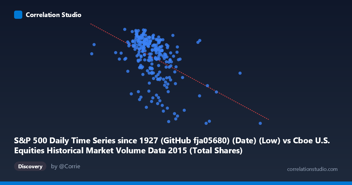
S&P 500 Daily Time Series since 1927 (GitHub fja05680) (Date) (Low) vs Cboe U.S. Equities Historical Market Volume Data 2015 (Total Shares)
- Pearson correlation (r)
- -0.4744
- Spearman correlation
- -0.4535
- p-value
- 0
- Sample size (n)
- 252
- 95% confidence interval
- -0.5649 to -0.3727
- Granger causality
- X → Y
- Granger optimal lag
- 5
AI analysis
Scatterplot Analysis: S&P 500 Daily Low vs. Cboe Total Shares Traded (2015)
Relationship Overview
The scatterplot reveals a negative relationship between the S&P 500 daily low price (X-axis) and total shares traded on U.S. equities exchanges (Y-axis) during 2015. As the index's daily low rises, total share volume tends to decline — a pattern consistent with the well-documented inverse relationship between equity prices and trading volume. Visually, the data form a downward-sloping cloud, with higher S&P 500 levels (roughly above 600M on the x-axis) associated with noticeably lower share counts, while lower price levels cluster around higher volume readings near 2,050–2,125 units.
Correlation Strength and Statistical Significance
The Pearson correlation of r = -0.4744 indicates a moderate negative association, but the explanatory power is modest: r² = 0.2251, meaning only about 22.5% of the variance in total shares traded is explained by the S&P 500 daily low. The remaining ~77.5% is attributable to other factors entirely. The 95% confidence interval of [-0.5649, -0.3727] is reasonably tight and does not cross zero, and the p-value of 1.554×10⁻¹⁵ confirms this is highly unlikely to be a chance finding across the sample of 252 paired observations drawn from a population of 3,302. Critically, the Granger causality analysis points in one direction: X (S&P 500 daily low) Granger-causes Y (total shares traded) with an optimal lag of 5 periods (F = 2.4148, p = 0.0369), while the reverse direction fails to reach significance (F = 0.3718, p = 0.8677). This suggests that S&P 500 price levels carry temporal predictive information about future trading volume, but volume does not meaningfully predict future price levels in this dataset.
Notable Patterns, Clusters, and Outliers
Several features stand out in the point distribution. The bulk of observations cluster between roughly 430M–560M on the X-axis and 2,040–2,130 on the Y-axis, suggesting the "normal" operating range of 2015 market conditions. However, a distinct lower-right cluster is visible — points above ~600M on X with Y values dipping toward 1,867–1,987 — corresponding to periods of elevated index prices coinciding with reduced share activity. A handful of outliers are conspicuous: the point near (208M, 2,059) sits far to the left of the main cluster, suggesting an anomalous low-price day with moderate volume, while points near (808M–815M, 1,867–1,971) represent the extreme high-price, low-volume end of the range. The spread of Y values at any given X level is also considerable, reinforcing that the linear fit, while statistically real, leaves substantial scatter unexplained.
Confounding Factors and Caveats
Several important caveats should temper interpretation. First, the axes appear to be swapped in the dataset labeling — the S&P 500 daily low is labeled as a "Date" column identifier and the volume metric carries the "Date" dataset label, suggesting potential metadata confusion worth verifying. Second, the S&P 500 price level is partly mechanical: higher nominal prices mean fewer shares are needed to achieve the same notional value, which could explain part of this inverse relationship arithmetically rather than behaviorally. Third, 2015 was a specific macro environment featuring late-cycle Federal Reserve tightening expectations and a summer volatility spike (August 2015), which may have driven simultaneous price drops and volume surges as a common response to external shocks — making both variables co-driven by a latent fear/uncertainty factor rather than causally linked to one another. The Granger result, while suggestive, does not establish true economic causality.
Actionable Insights and Further Investigation
Despite the moderate correlation, several avenues merit further exploration. The 5-period Granger lag deserves closer examination — analysts could construct a simple trading signal testing whether current S&P 500 price levels predict market activity roughly one week forward, useful for liquidity forecasting and execution strategy. It would also be valuable to decompose the volume metric by exchange or trade type (e.g., separating on-exchange from TRF volume) to determine whether the relationship holds uniformly or is driven by specific venues. Controlling for volatility (e.g., VIX or realized variance) as a confound would clarify how much of the relationship survives independently. Finally, extending the analysis across multiple years would test whether this pattern is structural or idiosyncratic to 2015's particular market dynamics, and whether the Granger predictive direction remains stable across different regimes.
X dataset: Cboe U.S. Equities Historical Market Volume Data 2015
Y dataset: S&P 500 Daily Time Series since 1927 (GitHub fja05680) (Date)
Part of experiment: Daily - Cboe U.S. Equities Historical Market Volume Data 2015 vs S&P 500 Daily Time Series since 1927 (GitHub fja05680) (Date)