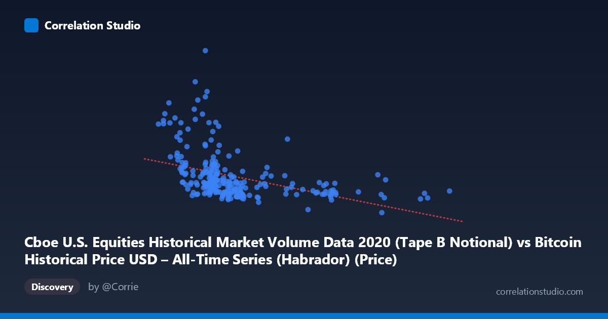
Cboe U.S. Equities Historical Market Volume Data 2020 (Tape B Notional) vs Bitcoin Historical Price USD – All-Time Series (Habrador) (Price)
- Pearson correlation (r)
- -0.4161
- Spearman correlation
- -0.5819
- p-value
- 0
- Sample size (n)
- 253
- 95% confidence interval
- -0.5131 to -0.3086
- Granger causality
- None
- Granger optimal lag
- 10
- Time coverage
- 2020-01-02 to 2020-12-31
- Recomputed on refreshed data
- 2026-10-24 (r was -0.4161)
AI analysis
Analysis: Cboe Equity Market Volume vs. Bitcoin Price (2020)
1. Overview of the Relationship
The scatterplot shows a moderate negative relationship between Cboe U.S. equities notional volume (X) and Bitcoin price (Y) across 253 paired daily observations from 2020. Most data points cluster tightly in the lower-left region — X values between roughly 7,000–12,000 and Y values between $4B–$8B — while a smaller number of high-Y outliers (Bitcoin prices above $10B... note the Y values appear to be scaled/notional, likely representing volume in dollars rather than literal BTC price) pull the trend downward as X increases. The bulk of the relationship is driven by this dense cluster, with a sparse tail of low-volume/high-price days.
2. Strength, Direction, and Statistical Confidence
The Pearson correlation of r = -0.416 indicates a modest negative linear association: as equity market volume increases, the paired value tends to decrease. However, r² = 0.173 means only 17.3% of the variance in Y is explained by X — the vast majority (over 82%) is driven by other factors entirely. The 95% CI [-0.513, -0.309] is reasonably tight and excludes zero, and the p-value (5.19E-12) confirms this correlation is highly statistically significant — not due to chance, given n=253. That said, statistical significance here reflects sample size and consistency, not necessarily practical strength or causal linkage.
Critically, the Granger causality tests show no significant predictive direction in either direction (X→Y: p=0.737; Y→X: p=0.361) at the optimal lag of 10 periods. This means neither variable reliably predicts the other's future values in a time-series sense — the correlation is contemporaneous/coincidental rather than a leading-lagging dynamic. This is an important caveat: correlation without Granger causality suggests both series may be responding to a shared external driver (e.g., macro market conditions, COVID-19 volatility in March 2020) rather than one influencing the other directly.
3. Notable Patterns and Outliers
Several observations stand out: - High-Y outliers at moderate-low X (e.g., X≈8,785 with Y≈$21.2B; X≈7,959 with Y≈$13.1B; X≈8,788 with Y≈$15.7B) appear to cluster around low X values (~5,800–9,800), suggesting a specific time period (likely the March 2020 COVID crash/volatility spike) where equity volumes were only moderately elevated but the Y-metric spiked dramatically. - High-X, low-Y points (X 17,000, e.g., 18,469–23,434) all correspond to compressed Y values ($3.7B–$5.4B), reinforcing the negative trend but with very few data points in this region — these could be leverage points disproportionately influencing the regression slope. - The relationship looks non-linear: dense, curved clustering suggests a possible logarithmic or power-law decay rather than a straight line, consistent with the note that Spearman ρ exceeds Pearson r.
4. Confounding Factors and Caveats
This pairing is unusual and warrants scrutiny: comparing 2020 equities volume to what's labeled a "Bitcoin price" series is a mismatched or possibly mislabeled dataset merge — the Y-axis metadata references "Price" but values in the billions suggest this is actually volume/notional data, not per-BTC price. This ambiguity should be resolved before drawing economic conclusions. Additionally: - Both series may be confounded by 2020's unique volatility regime (COVID crash in March, subsequent stimulus-driven rallies) — a period of extreme, correlated volatility across nearly all asset classes. - Small n (253) relative to population (4,254) means the sample may not evenly represent all trading days/regimes. - No lag/lead relationship (per Granger results) argues against a causal trading-flow story (e.g., "equity volume spikes drive crypto price moves" or vice versa).
5. Recommendations for Further Investigation
1. Verify data labeling — confirm whether Y truly represents Bitcoin price or mislabeled volume data, as this fundamentally changes interpretation. 2. Test non-linear models (log-linear, polynomial) given the Spearman/Pearson divergence — a log transform of X or Y may substantially improve fit. 3. Segment by regime (pre/post March 2020 crash) to check if the correlation is driven entirely by the volatility spike period rather than a stable year-round relationship. 4. Investigate shared confounders directly (e.g., VIX, overall market liquidity, stimulus announcements) rather than treating this as a bivariate relationship. 5. Given the lack of Granger causality, avoid using either series as a predictive signal for the other in trading models; treat the correlation as descriptive/contemporaneous only.
X dataset: Bitcoin Historical Price USD – All-Time Series (Habrador)
Y dataset: Cboe U.S. Equities Historical Market Volume Data 2020
Part of experiment: Bitcoin - Bitcoin Historical Price USD – All-Time Series (Habrador) vs Cboe U.S. Equities Historical Market Volume Data 2020