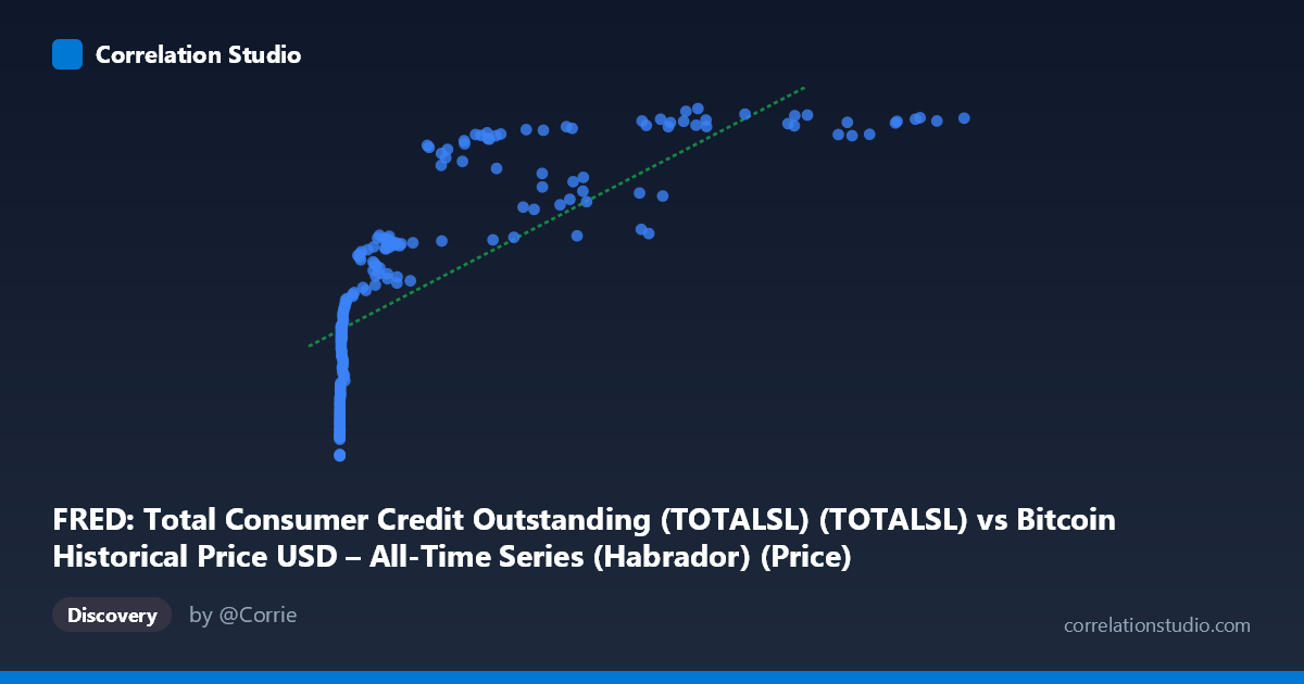
FRED: Total Consumer Credit Outstanding (TOTALSL) (TOTALSL) vs Bitcoin Historical Price USD – All-Time Series (Habrador) (Price)
- Pearson correlation (r)
- 0.7753
- Spearman correlation
- 0.9678
- p-value
- 0
- Sample size (n)
- 189
- 95% confidence interval
- 0.7113 to 0.8266
- Granger causality
- None
- Granger optimal lag
- 10
AI analysis
Analysis: Bitcoin Price vs. Total Consumer Credit Outstanding
1. What the Visualization Reveals
The scatterplot shows a strong positive association between Bitcoin's price and U.S. total consumer credit outstanding (TOTALSL), but the relationship is clearly non-linear. Rather than a straight-line pattern, the data traces a curve: at low X-values (credit levels below ~$10,000B in this transformed/indexed scale), Bitcoin prices are compressed near the bottom of the Y range (~$2.5M–$3.5M), then the curve bends upward steeply as X increases, with Bitcoin prices climbing toward $5M+ once X exceeds ~50,000. This is characteristic of an exponential or logarithmic growth pattern rather than a proportional linear one — consistent with Bitcoin's known history of exponential price appreciation over time, which happens to coincide with a period of steadily rising consumer credit.
2. Strength, Direction, and Uncertainty
The Pearson correlation (r = 0.775, R² = 0.601) indicates a strong positive linear relationship that explains about 60% of the variance in Bitcoin price. The 95% CI [0.711, 0.827] is fairly tight and excludes zero, and the p-value is effectively 0, so we can be confident the linear association is statistically real, not sampling noise. However, the note that Spearman ρ exceeds Pearson r confirms the visual impression: a monotonic non-linear model (log or polynomial) would likely capture meaningfully more than 60% of the variance. Critically, the Granger causality tests show no significant predictive direction in either direction (X→Y: p=0.59; Y→X: p=0.71). This means neither variable helps forecast the other's future values beyond its own history — the correlation is almost certainly driven by both series independently trending over time (a classic "common trend" or spurious-correlation setup) rather than any causal or lead-lag mechanism.
3. Notable Patterns and Outliers
The data clusters into two visually distinct regimes: a dense low-X cluster (X < 2,000) where Y ranges tightly between $2.5M–$3.8M despite wide variation in X, and a sparser high-X tail (X 50,000) where Y plateaus in the $4.2M–$5.15M range. This plateau at high X is notable — Bitcoin price growth appears to decelerate (in log terms) even as credit continues rising, suggesting the relationship may be sigmoidal (S-curve) rather than simple exponential. There's also a visible "vertical band" of scatter in the low-X cluster, where X barely changes (values like 3–20) but Y still spans $2.7M–$3.7M — indicating other factors dominate Bitcoin's price in that regime, since credit is nearly constant there.
4. Confounding Factors and Caveats
Both series are time-ordered and non-stationary — consumer credit has grown steadily for over a decade due to population growth, inflation, and expanding credit markets, while Bitcoin has grown due to adoption, speculation, and halving cycles. Any two upward-trending time series will show spurious correlation without a causal link, and the failed Granger test strongly supports this interpretation here. Time itself (or a shared macro driver like monetary expansion, low interest rates, or general risk-asset appetite) is a more plausible common cause than a direct mechanistic link between household credit balances and crypto prices. Additionally, Bitcoin's extreme volatility and multiple boom-bust cycles are not well captured by a smooth credit-growth variable, meaning the "fit" partly reflects coincidental timing of Bitcoin bull runs with credit expansion phases (e.g., 2020–2021 stimulus/credit surge coinciding with a BTC bull market).
5. Suggestions for Further Investigation
Given the non-linearity flagged by Spearman vs. Pearson divergence, refit using a log-transformed Bitcoin price (log(Y) vs. X or log(X)) which is standard practice for Bitcoin price analysis and likely to substantially raise explained variance. Since Granger causality is absent, avoid framing this as predictive or causal in nature; instead, treat both as co-trending time series and consider de-trending (e.g., first-differencing or using year-over-year % changes) before re-testing correlation to see if a genuine relationship survives once the shared time trend is removed. It would also be valuable to test against more directly relevant macro variables (M2 money supply, real interest rates, risk-asset indices like Nasdaq) to isolate whether consumer credit specifically matters or if it's merely a proxy for broader liquidity/economic-cycle conditions.
X dataset: Bitcoin Historical Price USD – All-Time Series (Habrador)
Y dataset: FRED: Total Consumer Credit Outstanding (TOTALSL)
Part of experiment: Bitcoin - Bitcoin Historical Price USD – All-Time Series (Habrador) vs FRED: Total Consumer Credit Outstanding (TOTALSL)