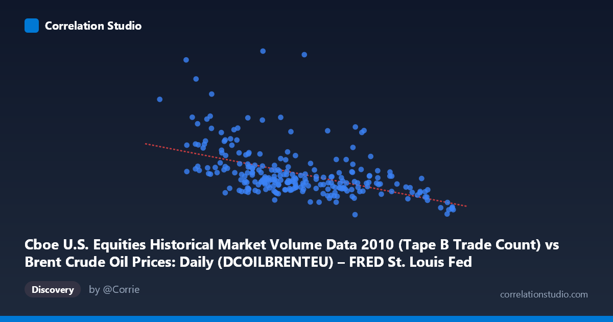
Cboe U.S. Equities Historical Market Volume Data 2010 (Tape B Trade Count) vs Brent Crude Oil Prices: Daily (DCOILBRENTEU) – FRED St. Louis Fed (DCOILBRENTEU)
- Pearson correlation (r)
- -0.4964
- Spearman correlation
- -0.5404
- p-value
- 0
- Sample size (n)
- 252
- 95% confidence interval
- -0.5842 to -0.3972
- Granger causality
- None
- Granger optimal lag
- 10
AI analysis
Analysis: Brent Crude Oil Price vs. Cboe Tape B Trade Count (2010)
Relationship Overview The scatterplot reveals a moderate negative relationship between Brent Crude Oil daily prices (X-axis, USD/barrel) and Cboe Tape B daily trade counts (Y-axis). The linear regression equation (y = -10,853.8x + 1,167,560) indicates that for each additional dollar per barrel in crude oil price, trade count decreases by approximately 10,854 units. Visually, the data cloud slopes downward from left to right, though with considerable scatter — days with lower oil prices (near $67–75/barrel) tend to show higher and more variable trade counts, while higher oil price days (near $85–93/barrel) cluster at lower, more compressed trade volumes.
Correlation Strength and Statistical Framing The Pearson correlation of r = -0.4964 indicates a moderate negative association, but the R² of 0.2464 is the more sobering metric: only 24.6% of the variance in trade count is explained by oil price alone, meaning roughly 75% of the variation is driven by other factors. The 95% confidence interval of [-0.5842, -0.3972] is meaningfully narrow and entirely negative, confirming directional consistency, and the p-value of ~0 (given N = 3,302) confirms this is not a chance artifact. However, the Granger causality results are notably absent in both directions — neither X→Y (F = 0.7524, p = 0.6744) nor Y→X (F = 0.8998, p = 0.5342) achieves significance at any conventional threshold. This is a critical finding: while a contemporaneous correlation exists, neither variable temporally predicts the other at the optimal 10-period lag, strongly cautioning against any causal narrative.
Patterns, Clusters, and Outliers Several features stand out in the data. There is a dense core cluster of points between roughly $75–85/barrel and 200,000–350,000 trades, suggesting a "typical" daily regime during mid-2010. However, the lower price range ($67–77/barrel) shows dramatically elevated variance, with trade counts spanning from ~200,000 to over 900,000 — the most extreme outlier being approximately (76.48, 918,659), which is nearly three standard deviations above the Y mean. Other high-trade-count days include (70.45, 778,566) and (47.00, 675,997), all clustering at lower oil prices. The high oil price range ($85–93/barrel) shows a tighter, lower cluster with counts generally below 400,000, suggesting reduced equity trading activity during periods of oil price elevation. This heteroscedasticity — widening variance at lower X values — is a meaningful structural feature that a simple linear model poorly captures.
Confounding Factors and Caveats Several confounds deserve serious consideration. Temporal autocorrelation is inherent in daily financial data — both oil prices and trade volumes exhibit momentum and regime-switching that can manufacture spurious correlations. The 2010 timeframe is historically specific: markets were still recovering from the 2008–2009 financial crisis, and oil prices were in a secular recovery trend (roughly $67 to $94 across the year), meaning the X-variable is partially a proxy for calendar time, conflating oil price effects with evolving post-crisis market structure. The Tape B designation (regional exchanges) adds complexity, as this segment's volume dynamics may reflect algorithmic trading patterns, exchange competition, or regulatory changes specific to 2010 rather than any fundamental oil-market sensitivity. Furthermore, the axis labels appear swapped in the dataset descriptions — the column naming is inverted between datasets — which warrants verification of which variable is genuinely "cause" and which is "effect" before any interpretation is finalized.
Actionable Insights and Further Investigation Given the moderate correlation without Granger causality, the most productive next steps would be to: (1) introduce time as an explicit covariate or use detrended/differenced series to isolate genuine co-movement from shared trends; (2) test for non-linear fits (e.g., polynomial or log-transformed Y), given the visible heteroscedasticity and the possibility that extreme trade volumes at low oil prices follow a different regime; (3) investigate the high-volume outliers individually — the ~5–6 days with trade counts above 500,000 likely correspond to identifiable market events (earnings seasons, macro announcements, or flash-crash-adjacent volatility episodes) that could explain the pattern far better than oil prices alone; and (4) expand the analysis to Tape A and C volumes to determine whether this relationship is specific to regional exchange activity or a broader market phenomenon. The correlation is real and statistically robust, but its practical utility for prediction or causal inference remains limited without deeper structural modeling.
X dataset: Brent Crude Oil Prices: Daily (DCOILBRENTEU) – FRED St. Louis Fed
Y dataset: Cboe U.S. Equities Historical Market Volume Data 2010
Part of experiment: Daily - Brent Crude Oil Prices: Daily (DCOILBRENTEU) – FRED St. Louis Fed vs Cboe U.S. Equities Historical Market Volume Data 2010