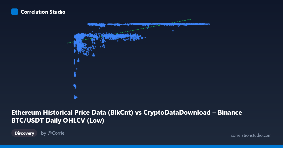
Ethereum Historical Price Data (BlkCnt) vs CryptoDataDownload – Binance BTC/USDT Daily OHLCV (Low)
- Pearson correlation (r)
- 0.5738
- Spearman correlation
- 0.7333
- p-value
- 0
- Sample size (n)
- 3191
- 95% confidence interval
- 0.5501 to 0.5966
- Granger causality
- None
- Granger optimal lag
- 1
- Time coverage
- 2017-08-17 to 2026-05-20
AI analysis
Analysis: X vs. Y Relationship
1. Overview of the Relationship
The scatterplot shows a positive but non-linear association between the X variable (labeled as an Ethereum block-count metric, though the value ranges suggest this may actually be BTC/USDT price data given the magnitudes) and Y (a price-like series ranging ~2,829–7,190). The data reveals a classic saturating/logarithmic curve: Y rises steeply as X increases from its minimum (~2,800) up to roughly 15,000–20,000, then flattens dramatically — with Y clustering tightly in a narrow 7,050–7,190 band for all X values above ~25,000, even as X stretches out to 123,000. This is not a straight-line relationship; it's a curve that plateaus.
2. Strength, Direction, and Statistical Confidence
The Pearson correlation (r = 0.574, r² = 0.329) indicates a moderate positive linear relationship, but the linear model only explains 32.9% of the variance in Y — meaning roughly two-thirds of Y's variability is left unexplained by a straight-line fit to X. The 95% CI [0.550, 0.597] is narrow and the p-value is effectively 0, so we can be confident some positive association exists and is not due to chance — but statistical significance here reflects the large sample size (n=3,191), not necessarily practical strength. Critically, the note that Spearman ρ exceeds Pearson r confirms what the scatterplot shows visually: the true relationship is monotonic but curved, and a log or polynomial fit would capture substantially more variance than the linear r² of 0.329 suggests. Finally, Granger causality tests show no significant predictive direction in either direction (X→Y: p=0.49; Y→X: p=0.86), meaning neither series' past values help forecast the other's future values at lag 1 — this is a contemporaneous/structural association, not a lead-lag or forecasting relationship.
3. Notable Patterns and Outliers
The most striking feature is the plateau effect: once X exceeds ~25,000–30,000, Y compresses almost entirely into the 7,100–7,190 range regardless of how much larger X gets (values up to 123,000). This suggests Y has a practical ceiling or saturation point. Conversely, the low-X region (X < 10,000) shows the most dispersion in Y (ranging from ~2,800 to ~6,500), indicating this is where the relationship is most dynamic and informative. A few low-X, low-Y points (e.g., X≈3,700–4,300, Y≈3,500–4,200) appear as a distinct lower cluster, possibly representing an early/different regime (e.g., an early time period or market phase) compared to the bulk of the data.
4. Confounding Factors and Caveats
Both series are financial/crypto time series, which are typically non-stationary, trending, and autocorrelated — this alone can inflate Pearson correlation without implying any causal or structural link (a well-known spurious correlation risk in time-series data covering 2017–2026, a period spanning multiple bull/bear cycles). The metadata is also inconsistent (X labeled as "Ethereum BlkCnt" but described as BTC/USDT OHLCV data; Y labeled as BTC "Low" price but under an "Ethereum" dataset title), so variable identity should be verified before drawing domain conclusions. Additionally, the ceiling effect in Y could reflect a bounded metric (e.g., a normalized price, a "Low" of a stablecoin-pegged pair, or a metric with a natural cap) rather than a true economic saturation — this needs domain context.
5. Recommendations for Further Investigation
Given the plateau shape and the Spearman-vs-Pearson discrepancy, refit the relationship using a log-transform of X or a piecewise/segmented regression to properly capture the low-X dynamic region and the high-X plateau separately — this should substantially raise explained variance beyond 32.9%. Since both variables are time series, run stationarity tests (ADF/KPSS) and consider differencing or detrending before computing correlation, to rule out spurious trend-driven association — the Granger non-causality result already hints that the raw-level correlation may not reflect meaningful dynamic linkage. Finally, clarify and correct the dataset/column labeling, and consider segmenting the analysis by time period (e.g., pre-2020 vs. post-2020) to check whether the relationship structure is stable across the different market regimes covered in this 2017–2026 span.
X dataset: CryptoDataDownload – Binance BTC/USDT Daily OHLCV
Y dataset: Ethereum Historical Price Data
Part of experiment: Bitcoin - CryptoDataDownload – Binance BTC/USDT Daily OHLCV vs Ethereum Historical Price Data