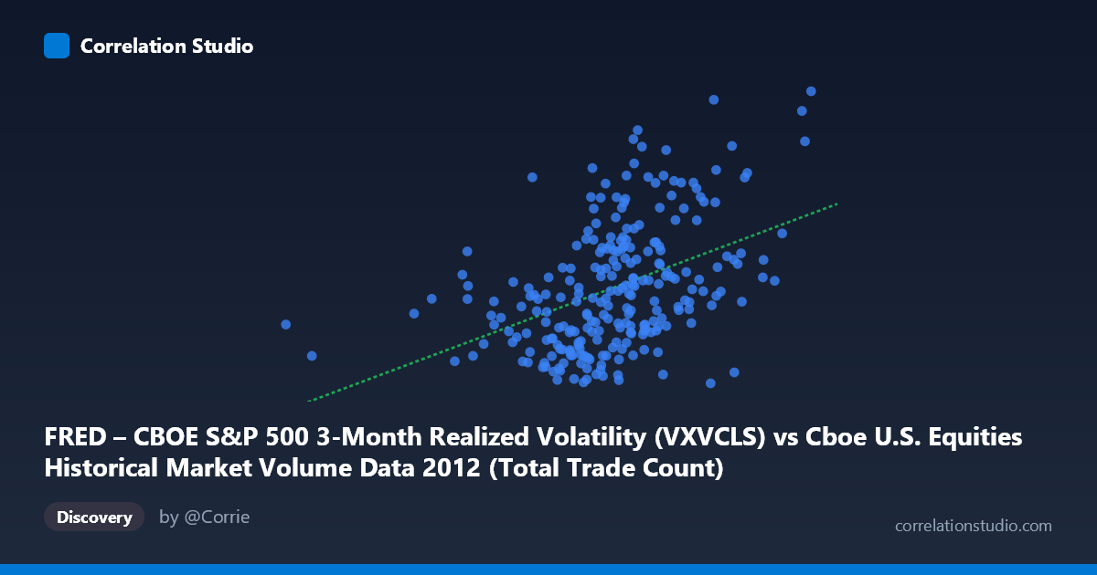
FRED – CBOE S&P 500 3-Month Realized Volatility (VXVCLS) vs Cboe U.S. Equities Historical Market Volume Data 2012 (Total Trade Count)
- Pearson correlation (r)
- 0.4383
- Spearman correlation
- 0.4571
- p-value
- 0
- Sample size (n)
- 250
- 95% confidence interval
- 0.3324 to 0.5334
- Granger causality
- None
- Granger optimal lag
- 1
AI analysis
Analysis: CBOE S&P 500 3-Month Realized Volatility vs. Total Trade Count (2012)
Relationship Overview
The scatterplot reveals a moderate positive relationship between CBOE S&P 500 3-month realized volatility (VXVCLS) and total U.S. equity trade counts during 2012. As volatility increases, trade counts tend to rise, which aligns intuitively with market microstructure theory: heightened uncertainty typically drives increased trading activity as investors rebalance, hedge, or react to price dislocations. The linear regression equation (y = 4.76E-06x + 12.55) confirms this positive slope, though the scatter around the regression line is substantial, suggesting the relationship is real but far from deterministic.
Correlation Strength and Statistical Significance
The correlation of r = 0.4383 indicates a moderate positive association, but the more telling statistic is r² = 0.1921 — meaning volatility explains only about 19.2% of the variance in trade counts. The remaining ~81% is attributable to other factors entirely. The 95% confidence interval [0.3324, 0.5334] is meaningfully above zero and relatively tight given n = 250, and the p-value of 3.67E-13 confirms the relationship is highly statistically significant — this is not a chance finding in a sample of this size. However, statistical significance should not be conflated with practical magnitude; the effect, while real, is modest. Critically, the Granger causality tests show no significant predictive direction in either direction (X→Y: F = 0.86, p = 0.36; Y→X: F = 0.42, p = 0.52), meaning that past volatility readings do not reliably predict future trade counts, and vice versa. The two variables move together contemporaneously but neither leads the other in a temporally exploitable way.
Notable Patterns, Clusters, and Outliers
Several features stand out in the sample data. There is a visible cluster of observations in the mid-volatility range (~18–22 Y-axis units) paired with trade counts concentrated between approximately 1.4M–1.9M, forming a dense core. However, there are notable high-volatility outliers — points such as (1,712,286, 25.50), (1,709,830, 26.50), and (1,737,562, 26.19) — where elevated volatility coincides with higher-than-average trade counts, pulling the regression slope upward. Conversely, some high-volume days (e.g., ~2.0–2.3M range) pair with only moderate volatility, suggesting episodic volume spikes driven by non-volatility factors such as index rebalancing, earnings events, or options expiration. The X range is notably wide [586K–2.28M], indicating considerable heterogeneity in daily trade counts throughout 2012.
Confounding Factors and Caveats
Several important caveats apply. First, reverse causality is plausible — high trade counts could themselves contribute to realized volatility calculations, creating circularity. Second, macro regime shifts in 2012 (e.g., European sovereign debt concerns, U.S. election, Fed policy announcements) likely created correlated spikes in both variables simultaneously, inflating the measured correlation without implying a structural relationship. Third, the VXVCLS measures 3-month implied volatility, which is a forward-looking market expectation — its alignment with contemporaneous trade counts blends two conceptually distinct time horizons. Fourth, day-of-week effects, options expiration cycles, and quarter-end rebalancing are systematic drivers of trade volume that are entirely independent of volatility, contributing to the large unexplained variance. Finally, the dataset covers only one calendar year, limiting generalizability.
Actionable Insights and Further Investigation
Despite the lack of Granger causality, the moderate contemporaneous correlation suggests that volatility regimes are worth monitoring as a soft signal for trading infrastructure capacity planning — high-volatility periods coincide with elevated trade volumes often enough to warrant preparedness. For deeper investigation, it would be valuable to: (1) segment the data by volatility quintile to test whether the relationship is linear or whether it accelerates above certain volatility thresholds; (2) introduce additional covariates such as VIX level, macroeconomic announcement days, and options expiration dates to isolate volatility's independent contribution; (3) extend the time series beyond 2012 to test whether this correlation is stable across different market regimes; and (4) explore nonlinear modeling approaches (e.g., regime-switching or quantile regression), given the visual scatter pattern suggests the relationship may strengthen materially at volatility extremes.
X dataset: Cboe U.S. Equities Historical Market Volume Data 2012
Y dataset: FRED – CBOE S&P 500 3-Month Realized Volatility
Part of experiment: Daily - Cboe U.S. Equities Historical Market Volume Data 2012 vs FRED – CBOE S&P 500 3-Month Realized Volatility