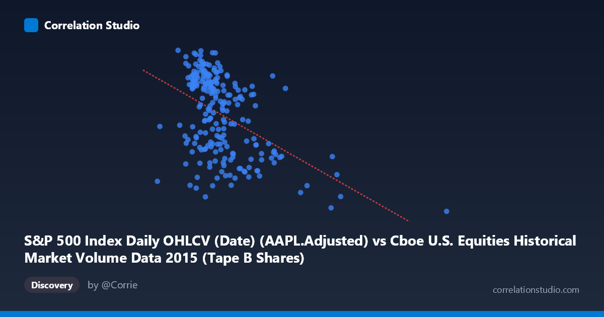
S&P 500 Index Daily OHLCV (Date) (AAPL.Adjusted) vs Cboe U.S. Equities Historical Market Volume Data 2015 (Tape B Shares)
- Pearson correlation (r)
- -0.4644
- Spearman correlation
- -0.4406
- p-value
- 0
- Sample size (n)
- 222
- 95% confidence interval
- -0.5617 to -0.3543
- Granger causality
- None
- Granger optimal lag
- 1
AI analysis
Scatterplot Analysis: AAPL Adjusted Price vs. Cboe Tape B Shares
1. Overall Relationship The scatterplot reveals a moderate negative relationship between Apple's adjusted stock price (X-axis) and Cboe Tape B share volume (Y-axis) over the 2015 trading year. As AAPL's adjusted price increases, Tape B shares traded tend to decrease, suggesting that periods of elevated AAPL valuation correspond with reduced activity in the Tape B market segment. The linear regression equation (y = -1.0664E-07x + 127.831) confirms this downward slope, though substantial scatter around the regression line is immediately apparent, indicating that the relationship is real but far from deterministic.
2. Correlation Strength and Statistical Significance The Pearson correlation of r = -0.4644 indicates a moderate negative association. However, the more practically meaningful statistic is r² = 0.2156, meaning AAPL's adjusted price explains only about 21.6% of the variance in Tape B share volume — leaving nearly 78% of variability attributable to other factors. The 95% confidence interval of [-0.5617, -0.3543] is reassuringly narrow and does not cross zero, and the p-value of 2.844E-13 confirms this correlation is highly statistically significant and extremely unlikely to be a chance artifact given n = 222 paired observations. That said, statistical significance here should not be conflated with practical importance, given the modest variance explained. Critically, Granger causality tests reveal no significant predictive directionality in either direction (X→Y: F = 0.635, p = 0.427; Y→X: F = 0.366, p = 0.546), meaning that past values of AAPL price do not meaningfully predict future Tape B volume, and vice versa. This rules out a simple lagged temporal mechanism and suggests the correlation reflects contemporaneous co-movement rather than a lead-lag relationship.
3. Notable Patterns, Clusters, and Outliers Several features stand out visually. The bulk of the data clusters between AAPL prices of roughly 70M–150M (likely representing adjusted price × volume scale or an index metric) with Tape B shares concentrated between 105–127, forming a discernible downward-sloping cloud. However, there are two prominent outliers at the high end of the X-axis: one point near (311.97M, 100.01) and another near (205M, 100.61), both exhibiting the lowest Tape B values in the dataset. These extreme observations likely correspond to specific high-volatility or high-price events in 2015 (possibly the August 2015 market selloff) and may be exerting disproportionate leverage on the regression slope, potentially inflating the apparent correlation. There also appears to be a non-linear pattern — the relationship may steepen dramatically at high X values, suggesting a threshold or regime-change effect rather than a purely linear one.
4. Confounding Factors and Caveats Several important caveats complicate interpretation. First, the axis labels appear inverted in the dataset metadata — the X variable is labeled as coming from the S&P 500 OHLCV dataset while the Y variable is from Cboe market volume data, suggesting potential dataset column assignment irregularities that warrant verification. Second, this is a time-series correlation spanning 2015-02-17 to 2015-12-31, meaning both variables may be simultaneously driven by macro market conditions (e.g., the August 2015 Chinese market shock, Federal Reserve rate speculation), creating spurious correlation through common external drivers rather than any direct relationship. Third, N = 506 population vs. n = 222 paired sample suggests approximately 56% of trading days could be matched — the reasons for missing pairs should be investigated as they may introduce selection bias. Finally, the absence of Granger causality at only a 1-period lag does not rule out longer-lag relationships.
5. Actionable Insights and Further Investigation Given these findings, several investigative steps are warranted. Outlier analysis should be prioritized — removing or Winsorizing the two extreme high-X observations and re-running the regression would clarify whether the correlation is robust or heavily outlier-driven. Non-linear modeling (e.g., polynomial regression or LOWESS smoothing) should be tested, as the cluster structure hints at a non-linear relationship. Expanding Granger causality tests to lags 2–10 would provide a more comprehensive picture of any delayed temporal effects. Additionally, introducing control variables such as the VIX (volatility index), overall S&P 500 daily returns, or broader market volume metrics would help isolate whether this correlation persists after accounting for shared macroeconomic drivers. Finally, verifying the dataset column assignments is essential before drawing any domain-specific conclusions.
X dataset: Cboe U.S. Equities Historical Market Volume Data 2015
Y dataset: S&P 500 Index Daily OHLCV (Date)
Part of experiment: Daily - Cboe U.S. Equities Historical Market Volume Data 2015 vs S&P 500 Index Daily OHLCV (Date)