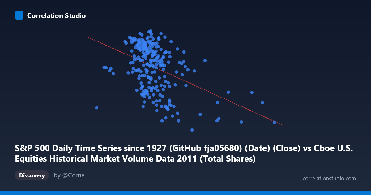
S&P 500 Daily Time Series since 1927 (GitHub fja05680) (Date) (Close) vs Cboe U.S. Equities Historical Market Volume Data 2011 (Total Shares)

Pearson correlation (r): -0.4229
Spearman correlation: -0.3747
p-value: 0
Sample size (n): 252
95% confidence interval: -0.5194 to -0.3159
Granger causality: None
Granger optimal lag: 1

AI analysis

Analysis: S&P 500 Closing Price vs. U.S. Equities Total Shares Traded (2011)

Relationship Overview The scatterplot reveals a moderate negative relationship between the S&P 500 daily closing price (X-axis) and total U.S. equities shares traded (Y-axis) across 2011. As the S&P 500 closing price increases, total trading volume tends to decrease — and conversely, periods of lower index prices are associated with higher share volumes. The linear regression equation (y = -2.15245E⁻⁷x + 1380.09) confirms this inverse slope, though the scatter around the regression line is considerable, indicating the relationship is real but far from deterministic.

Correlation Strength and Statistical Significance The Pearson correlation of r = -0.4229 indicates a moderate negative association. However, the coefficient of determination r² = 0.1789 means only about 17.9% of the variance in total shares traded is explained by the S&P 500 closing price level — leaving roughly 82% of variability attributable to other factors. The relationship is nonetheless highly statistically significant (p = 2.348E-12), and the 95% confidence interval of [-0.5194, -0.3159] is entirely negative, ruling out a chance positive or null correlation with high confidence. That said, statistical significance here is partly a function of the large sample (n = 252 from a population of 3,780), so the modest effect size deserves equal weight. Critically, Granger causality tests show no significant predictive directionality in either direction (X→Y: p = 0.9550; Y→X: p = 0.9702), meaning that despite the contemporaneous correlation, knowing today's S&P 500 price does not help predict tomorrow's trading volume, nor vice versa. This distinguishes a structural co-movement from any temporal lead-lag mechanism.

Notable Patterns, Clusters, and Outliers Several features stand out in the data. The bulk of observations cluster between roughly 400M–650M on the X-axis and 1,200–1,360 on the Y-axis, forming a relatively dense core. However, there is a visible right-side tail of higher X values (notably around 750M–880M and even ~1.2B) that tend to pull the regression downward, suggesting extreme high-volume days are associated with lower index prices — likely corresponding to the market stress periods of mid-to-late 2011. A handful of low-Y outliers (total shares ~1,100–1,165) at moderate X values around 588M–617M are also notable and may represent specific low-activity trading sessions. The distribution along X appears somewhat right-skewed given the mean (~522M) is well below the maximum (~1.2B), while Y values appear more normally distributed.

Confounding Factors and Caveats Several important caveats apply. First, 2011 was a particularly volatile year for equity markets, featuring the U.S. debt ceiling crisis, European sovereign debt fears, and the August S&P credit downgrade — all of which simultaneously depressed prices and spiked volume, creating a structural negative correlation that may not generalize to other periods. Second, the axes appear to be swapped relative to conventional intuition: the dataset labels suggest the S&P 500 date/close is used as the X variable while total shares is on Y, which is an unconventional pairing and worth verifying. Third, the negative correlation could partly reflect a long-term secular trend — both price and volume drift over time, and without detrending, the correlation may partially capture calendar-year drift rather than a pure contemporaneous relationship. Finally, the absence of Granger causality strongly cautions against any causal interpretation; this is a correlation between contemporaneous daily observations driven by shared macro forces, not a predictive signal.

Actionable Insights and Further Investigation Practitioners should treat this correlation as contextual rather than exploitable: high-volume days tend to coincide with market stress and lower prices in crisis-driven environments like 2011. For further investigation, it would be valuable to: (1) segment the data by market regime (e.g., pre- and post-August 2011 credit downgrade) to test whether the negative correlation is concentrated in stress periods; (2) test nonlinear specifications such as a log-log regression, given the right-skewed X distribution; (3) control for VIX or implied volatility as a mediating variable, since volatility simultaneously drives volume up and prices down; and (4) extend the analysis across multiple years to assess whether the r = -0.42 finding is a 2011-specific artifact or a persistent structural feature of U.S. equity market microstructure.

X dataset: Cboe U.S. Equities Historical Market Volume Data 2011

Y dataset: S&P 500 Daily Time Series since 1927 (GitHub fja05680) (Date)

Part of experiment: Daily - Cboe U.S. Equities Historical Market Volume Data 2011 vs S&P 500 Daily Time Series since 1927 (GitHub fja05680) (Date)