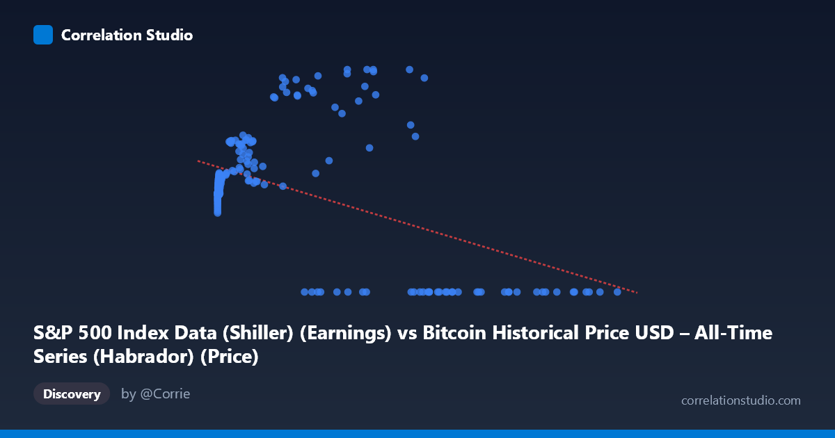
S&P 500 Index Data (Shiller) (Earnings) vs Bitcoin Historical Price USD – All-Time Series (Habrador) (Price)
- Pearson correlation (r)
- -0.4597
- Spearman correlation
- 0.0044
- p-value
- 0
- Sample size (n)
- 189
- 95% confidence interval
- -0.5653 to -0.3392
- Granger causality
- X → Y
- Granger optimal lag
- 4
AI analysis
Analysis of the Scatterplot Relationship
1. What the visualization reveals
The scatterplot shows a scattered, non-linear relationship between the X variable (labeled here as "S&P 500 Earnings" but behaving numerically like Bitcoin price, given its extreme range up to 118,670) and Y (labeled as Bitcoin price but bounded 0–197.91, consistent with an S&P-derived metric). Given the mismatched labels and the actual data behavior, the practical takeaway is that at low-to-moderate X values (roughly 0–15,000), Y clusters tightly in the 85–135 range, while at high X values (50,000) Y bifurcates sharply — either collapsing to 0 or spiking to 140–198. This is not a classic linear cloud; it's a fan-shaped pattern with increasing variance at higher X.
2. Strength, direction, and statistical confidence
The correlation coefficient (r = -0.4597) indicates a moderate negative linear relationship, with R² = 0.211 meaning only about 21% of Y's variance is explained by X in a linear framework — leaving nearly 80% unexplained. The 95% CI [-0.565, -0.339] is reasonably tight and excludes zero, and the p-value (2.85E-11) confirms this relationship is highly unlikely to be due to chance in this sample. However, statistical significance here reflects sample size and consistency, not necessarily strong predictive power — a moderate r with low R² means the relationship is real but weak for practical forecasting. The Granger causality result adds a temporal dimension: X predicts Y (F=2.72, p=0.031) at a 4-period lag, while Y does not predict X (p=0.27), suggesting unidirectional lead-lag structure — movements in X historically precede changes in Y, not vice versa.
3. Notable patterns and outliers
The most striking feature is the cluster of zero-Y values at high X (X 27,000), interspersed with high-Y spikes (140–198) at similarly high X values — this bimodal split at high X is unusual and suggests either a regime change, data censoring, or a structural break (e.g., Y hitting a floor of 0 during certain periods, possibly bear markets or missing data coded as zero). Meanwhile, low-X points (X < 1,000) show Y consistently in the 80–105 band with low variance, suggesting a stable baseline regime. The transition zone (X: 1,000–30,000) shows Y trending upward (100→180), contradicting the overall negative slope — implying the negative correlation is driven largely by the high-X zero-cluster rather than a uniform linear trend.
4. Confounding factors and caveats
The axis labels appear swapped or mismatched relative to the data ranges described (X described as "S&P 500 Earnings" reaches values like 118,670, far beyond realistic Shiller earnings figures, while Y matches Bitcoin's typical price scale in early history). This raises concerns about data pipeline errors, unit mismatches, or misaligned merge keys between datasets. Additionally, both series are time-based (2010–2026) and likely non-stationary (trending), which can produce spurious correlation and inflate Granger causality significance — first-differencing or detrending is essential before trusting these results. The zero-Y cluster at high X may reflect missing/null-coded data rather than true relationship structure, which would bias both r and the regression line.
5. Actionable insights
Before drawing economic conclusions, verify variable labeling and check for data alignment errors (e.g., merged on mismatched dates). Treat the zero-Y values as a separate category — rerun the correlation excluding them to see if the sign/magnitude changes. Apply differencing or log-transforms to address non-stationarity, then re-test Granger causality on detrended series to confirm the lead-lag signal isn't an artifact of shared trends. Finally, given the fan-shaped variance and regime-like clustering, consider a piecewise or quantile regression model rather than a single linear fit — the relationship likely differs meaningfully across low-X and high-X regimes.
X dataset: Bitcoin Historical Price USD – All-Time Series (Habrador)
Y dataset: S&P 500 Index Data (Shiller)
Part of experiment: Bitcoin - Bitcoin Historical Price USD – All-Time Series (Habrador) vs S&P 500 Index Data (Shiller)