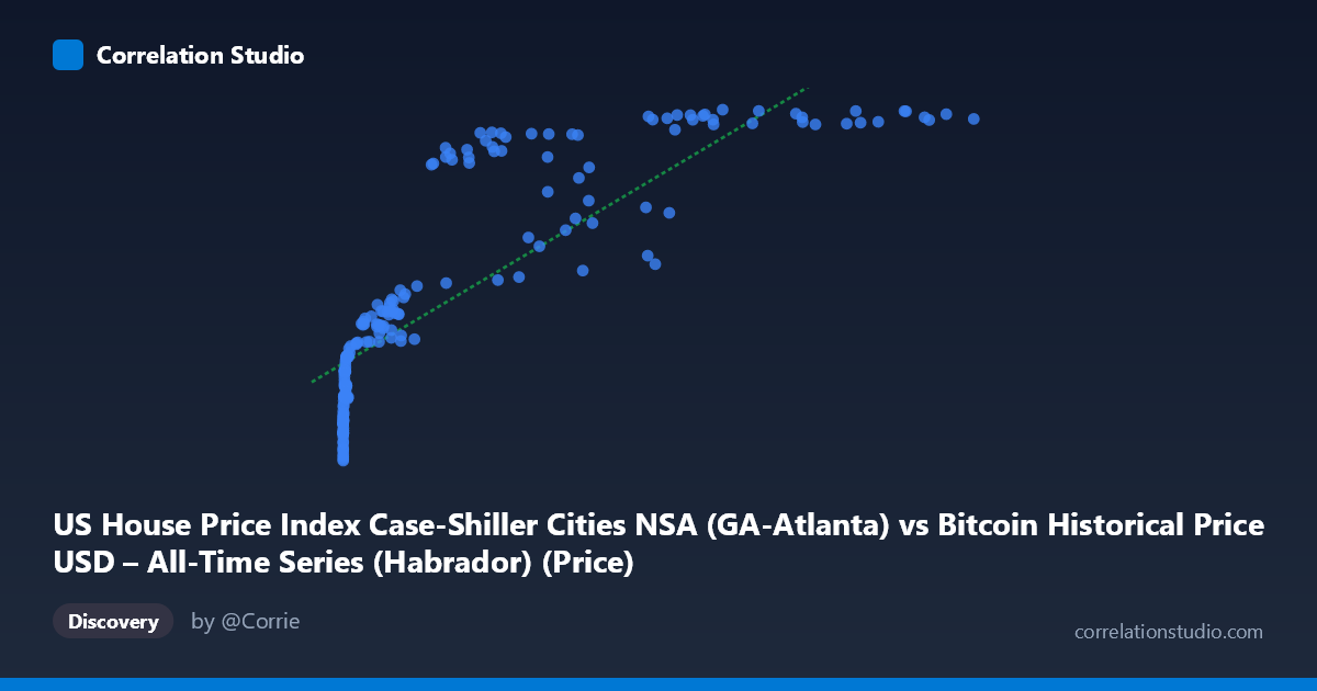
US House Price Index Case-Shiller Cities NSA (GA-Atlanta) vs Bitcoin Historical Price USD – All-Time Series (Habrador) (Price)
- Pearson correlation (r)
- 0.8332
- Spearman correlation
- 0.9644
- p-value
- 0
- Sample size (n)
- 187
- 95% confidence interval
- 0.7834 to 0.8724
- Granger causality
- None
- Granger optimal lag
- 1
AI analysis
Analysis: Bitcoin Price vs. Atlanta Case-Shiller Home Price Index
1. What the Visualization Reveals
The scatterplot shows a strong positive relationship between Bitcoin's historical USD price and the Atlanta Case-Shiller home price index, but this relationship is clearly non-linear. At low Bitcoin prices (under ~$1,000), the Atlanta HPI clusters tightly in the 85–140 range with steep sensitivity to small Bitcoin price changes. As Bitcoin climbs into the tens of thousands, the HPI compresses into a narrower band (roughly 240–252), producing a curve that resembles logarithmic or saturating growth rather than a straight line. This is essentially two time series that have both trended upward over the 2010–2026 window, creating a classic "spurious correlation via shared trend" pattern.
2. Strength, Direction, and Uncertainty
The Pearson correlation (r = 0.833) indicates a strong positive linear association, with r² = 0.694 meaning the linear model explains about 69% of the variance in Y. The 95% CI [0.783, 0.872] is tight and the p-value is effectively 0, so the correlation itself is statistically robust and not a sampling artifact. However, statistical significance here should not be mistaken for a meaningful causal or mechanistic link. The Granger causality tests are decisive on this point: neither direction shows significant predictive power (X→Y: p=0.25; Y→X: p=0.10). This means Bitcoin price history does not help forecast Atlanta home prices, nor vice versa — the correlation is contemporaneous/trend-driven, not temporally predictive.
3. Notable Patterns and Outliers
Several features stand out: - Compression at high X values: Once Bitcoin exceeds ~$50,000, HPI values saturate near 240–252, flattening the relationship — a strong sign of diminishing marginal association, not a true linear trend. - Steep low-end cluster: Below X=1,000, small Bitcoin price changes correspond to large jumps in HPI (e.g., X=0.06→106.4 vs. X=629→118.4), reflecting rapid house-price inflation during 2010–2013 while Bitcoin was still near-zero. - Non-monotonic dips: Points like (45,092, 174.69) and (56,973, 205.33) and (29,111, 170.10) fall well below the trend line compared to neighboring X values, likely corresponding to the 2022 Bitcoin crash/recovery period or HPI seasonal dips — evidence of cycle mismatches. - The note that Spearman ρ Pearson r confirms the rank-order relationship is stronger than the linear fit, reinforcing that a log or power-law transform of X would fit better.
4. Confounding Factors and Caveats
This is very likely a spurious correlation driven by mutual time trends rather than any economic mechanism linking Bitcoin speculation to Atlanta housing costs. Both series have risen over the 2010–2026 period due to entirely different macro drivers: Bitcoin due to adoption/speculative cycles and halving events, home prices due to low interest rates, inventory shortages, and regional demand in Atlanta specifically. Any two upward-trending time series will show inflated correlation. Additionally, comparing a highly volatile, globally-traded asset (Bitcoin) to a regionally-specific, smoothed monthly index (Case-Shiller) mixes vastly different volatility regimes and update frequencies, further distorting the apparent relationship. No adjustment for inflation, autocorrelation, or detrending appears to have been applied.
5. Suggestions for Further Investigation
- Detrend both series (e.g., first-differencing or removing a common time trend) and recompute correlation — this will likely reveal the "true" correlation is much weaker or negligible. - Log-transform Bitcoin price given its exponential growth pattern; this may improve linear fit and better reflect the diminishing-returns relationship suggested by the compression pattern. - Test against a national/broader HPI or a "typical" macro variable (M2 money supply, S&P 500) to see if Bitcoin correlates similarly with anything trending upward over this period — this would confirm the spurious-trend hypothesis. - Given the null Granger causality results, avoid using this pair for predictive modeling; treat the correlation as descriptive/historical co-movement only, not a forecasting signal.
X dataset: Bitcoin Historical Price USD – All-Time Series (Habrador)
Y dataset: US House Price Index Case-Shiller Cities NSA
Part of experiment: Bitcoin - Bitcoin Historical Price USD – All-Time Series (Habrador) vs US House Price Index Case-Shiller Cities NSA