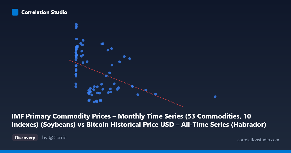
IMF Primary Commodity Prices – Monthly Time Series (53 Commodities, 10 Indexes) (Soybeans) vs Bitcoin Historical Price USD – All-Time Series (Habrador) (Price)
- Pearson correlation (r)
- -0.4471
- Spearman correlation
- -0.4437
- p-value
- 0.000023
- Sample size (n)
- 83
- 95% confidence interval
- -0.6045 to -0.256
- Granger causality
- None
- Granger optimal lag
- 10
AI analysis
Analysis: Bitcoin Price vs. Soybean Commodity Index
1. Overview of the Relationship
The scatterplot depicts a moderate negative association between soybean commodity prices (X-axis) and Bitcoin's historical USD price (Y-axis). The data shows a classic hyperbolic/decay pattern rather than a clean linear trend: a dense cluster of points sits at low X-values (0–50) spanning a wide range of Y-values (roughly 380–620), while sparser points extend out to X≈2452 with consistently low, compressed Y-values (330–530). This shape—high variance at low X, low variance at high X—is a strong visual signal that the linear correlation coefficient may be misleading.
2. Strength, Direction, and Statistical Confidence
The correlation is moderate and negative (r = -0.447), with r² indicating that only ~20% of the variance in one variable is explained by the other — meaning roughly 80% of the movement in Bitcoin's price is driven by factors unrelated to soybean prices (or vice versa). The 95% CI [-0.60, -0.26] is reasonably tight and entirely negative, and the p-value (2.27E-05) confirms this relationship is statistically significant and not due to chance. However, statistical significance here reflects the reliability of a weak-to-moderate effect, not its practical importance — 20% explained variance leaves substantial room for other drivers.
Critically, the Granger causality tests show no significant predictive direction in either direction (X→Y: p=0.354; Y→X: p=0.269). This means neither soybean prices nor Bitcoin prices reliably help forecast future values of the other over the tested lag structure (10 periods). This strongly suggests the correlation is contemporaneous/coincidental rather than causal — likely both series are independently trending over the 2010–2017 window (Bitcoin rising from near-zero, soybean index following its own commodity cycle) rather than one driving the other.
3. Notable Patterns and Outliers
The most striking feature is the dense vertical band near X=0–50, containing the majority of points and nearly the full Y-range (380–622). This suggests that for a long stretch of the sample period, soybean prices were compressed in a narrow low range while Bitcoin was highly volatile — consistent with Bitcoin's early speculative bull/bear cycles happening while soybean commodity prices were comparatively stable. Sparse "trailing" points at high X (997, 1089, 1230, 1402, 2452) all correspond to compressed Y-values (340–390), which have outsized leverage on the regression line/slope despite representing very few observations — a classic leverage/outlier concern.
4. Confounding Factors and Caveats
Both series are time-ordered economic variables, making them susceptible to spurious correlation via shared macro trends (USD strength, global risk sentiment, inflation expectations, general commodity/asset bull markets 2010–2017) rather than any direct economic linkage between Bitcoin and soybeans. The lack of Granger causality reinforces that this is likely not a causal relationship but rather two independent trends that happen to be modestly anti-correlated during this window. Additionally, the small sample (n=83 paired points from a population of 449) and uneven X-distribution (heavily skewed toward low values with a long right tail) mean the linear r/r² estimate is disproportionately influenced by a few high-leverage points, and a linear model is a poor fit for the visible curvature.
5. Recommendations for Further Investigation
Given the visual hyperbolic shape, a log-transform of X (or both variables) and re-fitting would likely produce a more honest and possibly stronger fit than the linear model's 20% R². Researchers should treat this pairing as a spurious/coincidental correlation absent causal evidence, and instead investigate shared underlying macro drivers (e.g., USD index, global liquidity/interest rates, general risk-on/risk-off sentiment) that could simultaneously affect both crypto and agricultural commodity markets. Finally, given Granger non-significance, this pairing has limited value for predictive/trading models linking soybean futures to Bitcoin price movements — resources are better directed toward assets with demonstrated lead-lag structure.
X dataset: Bitcoin Historical Price USD – All-Time Series (Habrador)
Y dataset: IMF Primary Commodity Prices – Monthly Time Series (53 Commodities, 10 Indexes)
Part of experiment: Bitcoin - Bitcoin Historical Price USD – All-Time Series (Habrador) vs IMF Primary Commodity Prices – Monthly Time Series (53 Commodities, 10 Indexes)