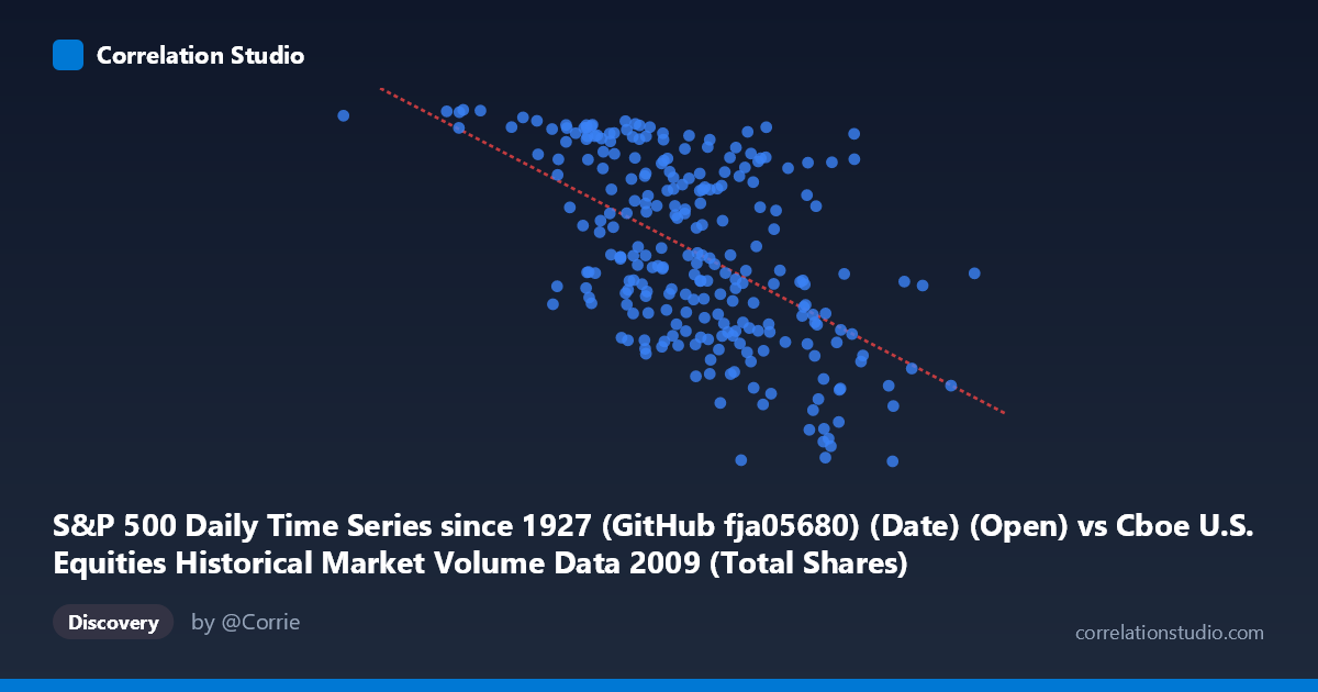
S&P 500 Daily Time Series since 1927 (GitHub fja05680) (Date) (Open) vs Cboe U.S. Equities Historical Market Volume Data 2009 (Total Shares)
- Pearson correlation (r)
- -0.5548
- Spearman correlation
- -0.5463
- p-value
- 0
- Sample size (n)
- 252
- 95% confidence interval
- -0.6349 to -0.463
- Granger causality
- X → Y
- Granger optimal lag
- 10
AI analysis
Analysis: S&P 500 Open Price vs. Cboe Total Shares Volume (2009)
1. Relationship Overview The scatterplot reveals a moderate negative relationship between the S&P 500 daily open price (X-axis) and total U.S. equity shares traded on Cboe exchanges (Y-axis) across the 2009 trading year. As the S&P 500 open price increases, total daily share volume tends to decline. This is visually consistent with the broader narrative of 2009: early in the year, prices were severely depressed (post-financial crisis lows near 680–750 range) while panic-driven trading activity was elevated, and as prices recovered through the year, the urgency to trade—and thus volume—gradually subsided.
2. Correlation Strength, Direction, and Causality The Pearson correlation of r = −0.5548 indicates a moderate negative association, but the explained variance figure tells a more measured story: r² = 0.3078 means only ~30.8% of the variance in total share volume is explained by the S&P 500 open price. This leaves roughly 70% of volume variability attributable to other factors entirely. The 95% confidence interval of [−0.6349, −0.4630] is meaningfully narrow given n = 252, and the p-value of effectively zero confirms this relationship is not a statistical artifact—it is a reliable signal within this sample. Critically, Granger causality runs unidirectionally from X→Y (F = 2.31, p = 0.0134), meaning lagged S&P 500 open prices carry statistically significant predictive information about future share volume at an optimal lag of 10 trading periods (~2 calendar weeks). The reverse direction (Y→X) fails to reach significance at conventional thresholds (p = 0.0748), suggesting volume does not meaningfully predict future prices in this dataset—a non-trivial finding for market practitioners.
3. Notable Patterns, Clusters, and Outliers Several structural features stand out in the data. There is a visible cluster of high-volume, low-price observations in the lower-right-to-lower-left zone (prices ~680–800, volumes ~679–860 million shares), corresponding to the market's distressed trough in early 2009. A second loose cluster appears at mid-to-high prices (~900–1,100) with more dispersed, moderate volume levels, reflecting the recovery phase. Outliers worth flagging include the point at approximately (1,212,524,831, 919.58)—the highest price observation—which shows only moderate volume, and (192,269,943, 1,121.08), the lowest price observation, which pairs with very high volume. The point at (1,080,132,313, 679.28) represents the minimum volume in the sample despite being at a relatively high price, suggesting a notable anomaly possibly tied to a holiday-shortened session or a specific market event. The relationship also exhibits heteroscedasticity: variance in volume is considerably wider at mid-range price levels than at the extremes, hinting that a linear model may be oversimplifying the true functional form.
4. Confounding Factors and Interpretive Caveats Several important caveats apply. First, 2009 is a regime-specific year—it encompasses one of the most dramatic bear-market bottoms (March 2009) and a sharp recovery, making price and volume dynamics unusually co-determined by macroeconomic fear and sentiment rather than ordinary market mechanics. The correlation likely reflects a shared driver (crisis severity) rather than a direct causal mechanism between price level and volume per se. Second, the linear regression equation (y = −4.11×10⁻⁷x + 1,259.82) implies a very shallow slope given the enormous X-axis scale (hundreds of millions), which underscores that the practical magnitude of the price effect on volume per unit is tiny in absolute terms. Third, temporal autocorrelation in both price and volume series is nearly certain in daily financial data, which can inflate apparent correlation and inflate the significance of the Granger test if not fully controlled. Finally, the N = 3,232 population size versus n = 252 sample raises questions about whether the sampled days are representative of the full intraday or tick-level data population from which they were drawn.
5. Actionable Insights and Further Investigation The Granger causality result is the most actionable finding here: S&P 500 open prices at a 10-day lag appear to carry predictive signal for Cboe share volume, which could be incorporated into volume-forecasting models for liquidity planning, execution strategy, or market-making. Practitioners should investigate whether this predictive lag is stable across other years or specific to crisis-recovery regimes. It would be worthwhile to test a non-linear or piecewise specification (e.g., segmenting by market regime or fitting a quadratic/logarithmic model), given the visual heteroscedasticity and the theoretical expectation that volume-price relationships are asymmetric around market extremes. Additionally, controlling for the VIX or other volatility proxies as covariates would help isolate whether price level itself drives volume or whether both are jointly driven by investor fear. Expanding the time window beyond 2009 would test whether this relationship is structurally persistent or an artifact of extraordinary market conditions.
X dataset: Cboe U.S. Equities Historical Market Volume Data 2009
Y dataset: S&P 500 Daily Time Series since 1927 (GitHub fja05680) (Date)
Part of experiment: Daily - Cboe U.S. Equities Historical Market Volume Data 2009 vs S&P 500 Daily Time Series since 1927 (GitHub fja05680) (Date)