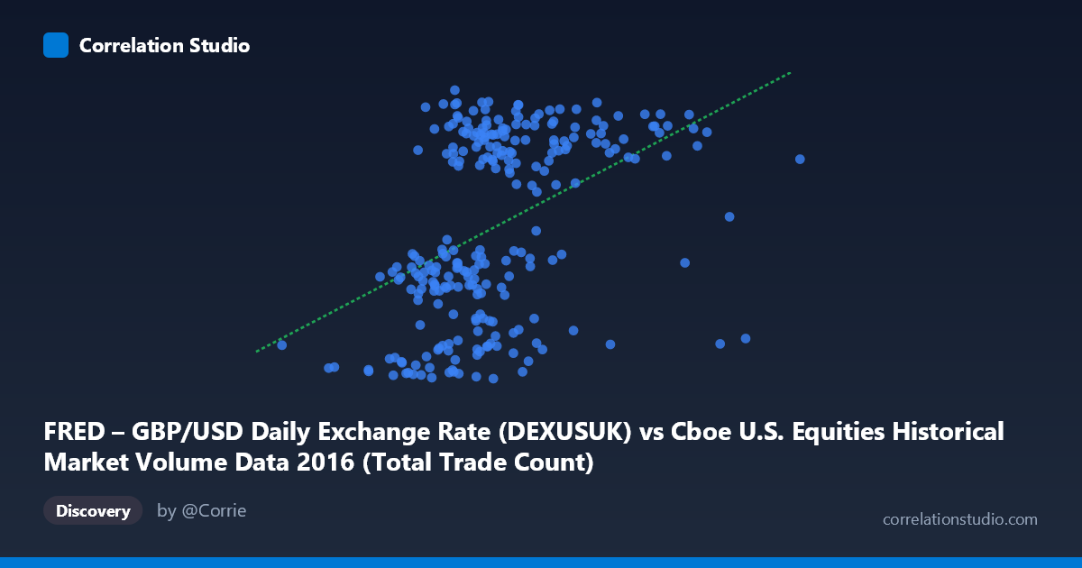
FRED – GBP/USD Daily Exchange Rate (DEXUSUK) vs Cboe U.S. Equities Historical Market Volume Data 2016 (Total Trade Count)
- Pearson correlation (r)
- 0.4336
- Spearman correlation
- 0.4644
- p-value
- 0
- Sample size (n)
- 250
- 95% confidence interval
- 0.3271 to 0.5292
- Granger causality
- None
- Granger optimal lag
- 1
AI analysis
Analysis: GBP/USD Exchange Rate vs. U.S. Equities Total Trade Count (2016)
Relationship Overview The scatterplot reveals a modest positive relationship between Cboe U.S. equity market total trade counts and the GBP/USD exchange rate across 2016. As daily trade volume (measured by total trade count) increases, the pound tends to trade at a slightly higher value against the dollar. The linear regression equation (y = 6.95E-08x + 1.1869) suggests a very small but positive slope — for every one-unit increase in trade count, the GBP/USD rate increases by roughly 0.0000000695. While statistically detectable, this effect is numerically tiny, and the wide scatter visible around the regression line immediately signals that the relationship is far from deterministic.
Correlation Strength and Statistical Framing The Pearson correlation of r = 0.4336 indicates a weak-to-moderate positive association. More telling is the r² value of 0.1880, meaning that trade count explains only 18.8% of the variance in GBP/USD — leaving over 81% attributable to other factors entirely. The 95% confidence interval for r [0.3271, 0.5292] is reasonably tight given n = 250, and the p-value of 7.01E-13 confirms the correlation is highly statistically significant, effectively ruling out chance as an explanation with this sample size. However, statistical significance here is largely a function of the large population (N = 3,622) rather than a strong effect size. Crucially, Granger causality tests find no significant predictive direction in either direction — neither X→Y (F = 0.071, p = 0.790) nor Y→X (F = 0.449, p = 0.503) — meaning that past values of trade count do not help predict future GBP/USD levels, and vice versa. This decisively undermines any practical trading or forecasting application of this correlation.
Notable Patterns, Clusters, and Outliers Several structural features are visible in the sample data. The Y-axis (GBP/USD) clusters into two loosely distinct bands: a lower band approximately between 1.22–1.35 and an upper band between 1.38–1.48, with a relative gap in between. This bimodal-like distribution in Y strongly suggests a structural break or regime shift during 2016 — almost certainly the Brexit referendum on June 23, 2016, which caused a dramatic and sustained drop in sterling. On the X-axis, most trade counts concentrate between roughly 1.6M and 3.0M, but several pronounced outliers extend to ~3.96M and ~4.14M. These high-volume outliers (e.g., the points near X = 3,963,608 and 4,139,281) correspond to GBP/USD values of only ~1.25, consistent with post-Brexit elevated volatility and trading activity occurring when sterling was depressed.
Confounding Factors and Interpretation Caveats The most significant caveat is that 2016 was an extraordinary year for GBP/USD due to Brexit, creating a non-stationary time series with a structural break mid-year. Any correlation measured across the full year conflates two distinct regimes (pre- and post-Brexit), inflating or distorting the apparent relationship. Additionally, U.S. equity trade counts are influenced by entirely independent drivers — earnings seasons, U.S. economic data, Federal Reserve decisions, and domestic volatility events — which have no direct link to sterling dynamics. The correlation likely reflects a common driver: global risk-off sentiment and volatility spikes simultaneously depressed GBP (risk-sensitive currency) and elevated U.S. equity trading volumes. This is a classic spurious correlation mediated by a third variable (market-wide risk appetite or the VIX), rather than any direct causal mechanism between the two series.
Actionable Insights and Further Investigation Given the absence of Granger causality, this relationship should not be used for predictive modeling in either direction. However, several follow-up analyses would be valuable: (1) Split the dataset at the Brexit date (June 23, 2016) and compute correlations separately for pre- and post-Brexit subperiods to test whether the relationship is regime-dependent; (2) Introduce a volatility proxy such as the VIX or VVIX as a control variable in a multivariate regression to test whether the correlation vanishes once common risk sentiment is accounted for; (3) Examine trade count by exchange type (e.g., Cboe BZX vs. TRFs) to determine whether the signal is concentrated in specific venues associated with cross-asset arbitrage or ETF activity; and (4) consider rolling-window correlation analysis to visualize how the r value evolved through the year, which would likely reveal a structural shift around mid-June 2016 and provide a cleaner picture of the true underlying dynamics.
X dataset: Cboe U.S. Equities Historical Market Volume Data 2016
Y dataset: FRED – GBP/USD Daily Exchange Rate
Part of experiment: Daily - Cboe U.S. Equities Historical Market Volume Data 2016 vs FRED – GBP/USD Daily Exchange Rate