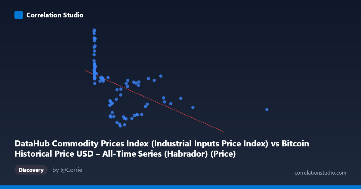
DataHub Commodity Prices Index (Industrial Inputs Price Index) vs Bitcoin Historical Price USD – All-Time Series (Habrador) (Price)
- Pearson correlation (r)
- -0.5156
- Spearman correlation
- -0.7451
- p-value
- 0.000001
- Sample size (n)
- 83
- 95% confidence interval
- -0.6581 to -0.3374
- Granger causality
- None
- Granger optimal lag
- 1
AI analysis
Analysis of the Scatterplot Relationship
1. What the Visualization Reveals
The scatterplot shows a downward-sloping but noisy relationship between two labeled variables (note the axis labels appear swapped in the metadata — X is described as a commodity price index while its data range [0.06–2452.18] and sample values actually resemble Bitcoin's historical price trajectory, and Y's tight range [105–217] resembles a commodity index). Regardless of labeling, the pattern shows a dense cluster of points at low X values (roughly 0–50) with Y values spread across the full range (155–217), followed by a long, sparse tail extending to X≈2452 where Y values consistently sit in a lower band (105–160). This creates the visual impression of an inverse relationship, but it is driven largely by the structure of the tail rather than a uniform linear trend throughout.
2. Strength, Direction, and Statistical Confidence
The correlation is moderate and negative (r = -0.5156), with r² = 0.2658 indicating that only about 27% of the variance in Y is explained by X — meaning roughly 73% of Y's variability is driven by other factors entirely. The 95% confidence interval [-0.658, -0.337] is reasonably tight and excludes zero, and the p-value (6.1×10⁻⁷) confirms this correlation is highly unlikely to be due to chance. However, statistical significance should not be conflated with practical strength: this is a real but modest relationship, not a tight coupling. Critically, the Granger causality tests show no significant predictive direction in either direction (X→Y: p=0.399; Y→X: p=0.692), meaning that despite the contemporaneous correlation, neither series helps forecast the other's future values based on past values. This strongly suggests the relationship is either coincidental co-trending, driven by a shared external factor, or a spurious correlation from overlapping macro-trends rather than a genuine causal or lead-lag mechanism.
3. Notable Patterns and Outliers
The data is highly heteroscedastic: variance in Y is much larger at low X (spanning ~155–217) and compresses substantially at high X (settling into a narrower 105–160 band). This funnel shape violates the constant-variance assumption of simple linear regression and inflates the apparent linear fit at the extremes while the linear model poorly captures the dense low-X cluster. The note that Spearman ρ exceeds Pearson r reinforces that a monotonic but non-linear (e.g., logarithmic or power-law decay) relationship fits better — consistent with the pattern of a steep initial drop in Y as X moves from 0 to ~500, followed by a flattening/plateau for X 500. A few high-leverage points near X≈2452 and X≈1400 sit far from the main mass of data and disproportionately influence the linear slope estimate.
4. Confounding Factors and Caveats
Both series span 2010–2017, a period during which Bitcoin price and broad commodity indices were each independently trending due to distinct macro cycles (Bitcoin's speculative bull/bear cycles vs. commodity supercycles tied to global growth, USD strength, and China demand). Any two non-stationary time series with long-term trends can show spurious correlation without genuine linkage — this is a classic case where time itself is a likely confounder. The lack of Granger causality supports this: the correlation may simply reflect that Bitcoin trended upward while commodities cooled over this window, not a causal or reactive market relationship. Additionally, n=83 paired points sampled from a larger population (N=449) may not evenly represent the full time series, and irregular time sampling of Bitcoin's exponential price growth could distort the correlation structure.
5. Suggestions for Further Investigation
Given the non-linear signal (Spearman Pearson), refitting with a log-transform on X (given its extreme right-skew, ranging over 4 orders of magnitude) would likely improve fit and better satisfy linearity/homoscedasticity assumptions. Because both series may be non-stationary trending time series, analysts should test for unit roots and consider using differenced or detrended series (or cointegration analysis) rather than raw levels to distinguish genuine co-movement from shared trend artifacts. Given the null Granger causality result, this correlation should not be used for predictive/trading purposes; instead, treat it as a descriptive historical association and investigate plausible shared macro drivers (e.g., USD index, global risk sentiment, inflation expectations) that might independently explain both series' trajectories over 2010–2017.
X dataset: Bitcoin Historical Price USD – All-Time Series (Habrador)
Y dataset: DataHub Commodity Prices Index
Part of experiment: Bitcoin - Bitcoin Historical Price USD – All-Time Series (Habrador) vs DataHub Commodity Prices Index