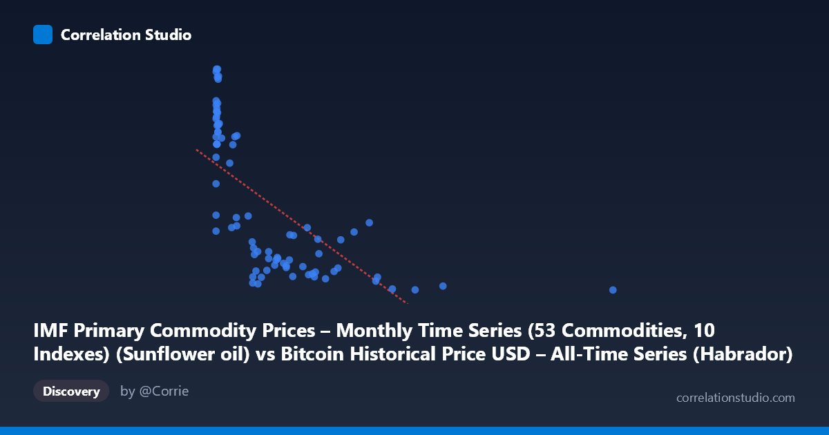
IMF Primary Commodity Prices – Monthly Time Series (53 Commodities, 10 Indexes) (Sunflower oil) vs Bitcoin Historical Price USD – All-Time Series (Habrador) (Price)
- Pearson correlation (r)
- -0.6685
- Spearman correlation
- -0.7879
- p-value
- 0
- Sample size (n)
- 83
- 95% confidence interval
- -0.7728 to -0.5291
- Granger causality
- None
- Granger optimal lag
- 10
- Time coverage
- 2010-08-01 to 2017-06-01
AI analysis
Analysis of Bitcoin Price vs. Sunflower Oil Commodity Index
1. What the Visualization Reveals
The scatterplot shows a moderately strong inverse relationship between sunflower oil prices (X-axis) and Bitcoin price in USD (Y-axis). At low sunflower oil values (roughly 0–20), Bitcoin prices span a wide range, from ~1140 to over 1700, with many high-value clusters. As sunflower oil prices increase beyond ~200–300, Bitcoin prices compress into a much narrower, lower band (roughly 950–1150). This produces a curved, decaying pattern rather than a straight diagonal line — consistent with the note that Spearman's ρ exceeds Pearson's r, hinting at a non-linear (possibly logarithmic or power-law) decay rather than a strictly linear decline.
2. Strength, Direction, and Statistical Confidence
The Pearson correlation of r = -0.6685 indicates a moderately strong negative linear association, with r² = 0.447 meaning sunflower oil prices statistically explain about 45% of the variance in Bitcoin prices in this sample — leaving the majority (55%) unexplained by this variable alone. The 95% confidence interval [-0.773, -0.529] is fairly tight and entirely negative, and the p-value (4.99e-12) is highly significant, giving strong confidence that a real (non-zero) negative association exists in the underlying data-generating process, not just sampling noise.
However, the Granger causality tests reveal no significant predictive direction in either direction (X→Y: p=0.509; Y→X: p=0.169). This is a critical caveat: despite the strong contemporaneous correlation, neither variable helps forecast future movements of the other over time. This strongly suggests the relationship is not causal in a temporal/predictive sense — it's more likely a shared association with a common underlying driver (e.g., both series reflect long-term secular trends over the 2010–2017 window) rather than one variable mechanically influencing the other.
3. Notable Patterns and Outliers
The data reveals a dense cluster at very low X values (X < 20) where Y ranges dramatically (1140 to 1700+) — this is the region driving most of the variance and where Bitcoin's early volatile price history (2010–2013) is concentrated. A second, tighter cluster appears at moderate-to-high X (300–1400) with Y compressed near 950–1150, representing a later, calmer Bitcoin price era. There's also a clear outlier/leverage point at X=2452.18, Y=936.24 — an extreme sunflower oil value far beyond the rest of the distribution, which likely has outsized influence on the regression slope. The overall shape resembles an inverse or log-decay curve rather than a line, which explains the R² gap between Pearson and Spearman measures.
4. Confounding Factors and Caveats
This is almost certainly a spurious or confounded correlation driven by time. Both series are time-indexed (2010–2017), and Bitcoin's price trajectory is dominated by its own idiosyncratic adoption/bubble cycles, while sunflower oil prices are driven by agricultural supply/demand, weather, and global commodity cycles — there's no plausible direct economic mechanism linking them. The correlation likely emerges because both variables have long-term trends (rising commodity prices post-2010, then Bitcoin's later divergent rally) that happen to move in opposite directions over this window purely coincidentally. The lack of Granger causality reinforces that this is a level/trend correlation, not a dynamic relationship — a hallmark of two unrelated non-stationary time series.
5. Suggested Next Steps
Analysts should detrend or difference both series (e.g., analyze month-over-month % changes rather than raw levels) and recompute correlation — true economic relationships should survive detrending, whereas spurious trend-driven correlations typically vanish. Fitting a log or power-law model to X may improve fit given the Spearman/Pearson gap, but this should be checked for robustness by excluding the extreme outlier (X=2452). Given the null Granger causality result, this pairing should not be used for forecasting purposes; instead, treat both series as independently trending and consider testing against genuine macro drivers of Bitcoin (e.g., USD index, risk-asset sentiment, regulatory events) rather than an agricultural commodity with no direct linkage.
X dataset: Bitcoin Historical Price USD – All-Time Series (Habrador)
Y dataset: IMF Primary Commodity Prices – Monthly Time Series (53 Commodities, 10 Indexes)
Part of experiment: Bitcoin - Bitcoin Historical Price USD – All-Time Series (Habrador) vs IMF Primary Commodity Prices – Monthly Time Series (53 Commodities, 10 Indexes)