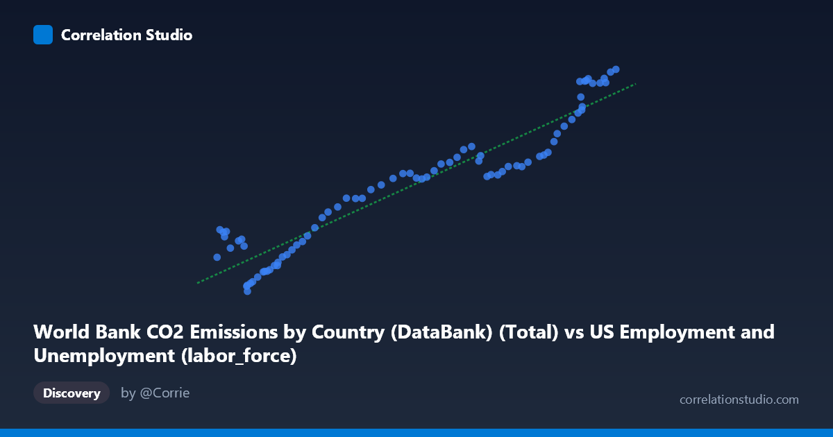
World Bank CO2 Emissions by Country (DataBank) (Total) vs US Employment and Unemployment (labor_force)
- Pearson correlation (r)
- 0.9493
- Spearman correlation
- 0.9334
- p-value
- 0
- Sample size (n)
- 80
- 95% confidence interval
- 0.9218 to 0.9673
- Granger causality
- None
- Granger optimal lag
- 10
- Time coverage
- 1941-01-01 to 2020-01-01
AI analysis
Scatterplot Analysis: US Labor Force vs. CO2 Emissions
1. Overall Relationship
The scatterplot reveals a strong, predominantly positive linear relationship between total CO2 emissions and the US labor force size across the period 1941–2020. As CO2 emissions increase, labor force participation grows correspondingly, tracing a broadly upward trajectory consistent with decades of simultaneous economic and demographic expansion. The fitted regression line (y = 0.2477x − 889.56) captures this trend well across most of the data range, suggesting that both variables are jointly driven by long-run economic growth dynamics rather than one directly causing the other.
2. Correlation Strength and Statistical Interpretation
The Pearson correlation of r = 0.9493 is exceptionally strong, and the R² of 0.9011 indicates that approximately 90.1% of the variance in labor force size is statistically accounted for by CO2 emissions within this linear model — a remarkably high figure for macroeconomic data spanning eight decades. The 95% confidence interval [0.9218, 0.9673] is narrow, confirming high precision in the estimate, and the p-value of effectively zero eliminates any concern about chance association at conventional significance thresholds. However, the Granger causality analysis critically undermines any causal narrative: neither direction (X→Y: F = 0.9595, p = 0.490; Y→X: F = 1.0736, p = 0.400) reaches statistical significance at lag 10, meaning that past values of CO2 emissions do not meaningfully predict future labor force levels, and vice versa. This firmly situates the relationship as correlational and likely spurious — two parallel trends driven by shared underlying forces rather than any direct temporal predictive linkage.
3. Notable Patterns, Clusters, and Outliers
Several structural features are visible in the data. A dense lower-left cluster (roughly X: 53,000–75,000; Y: 10,000–19,000) corresponds to earlier decades with lower emissions and smaller labor forces, where some scatter is evident — points like (54,630; 19,109) and (53,860; 14,971) sit somewhat above the regression line, suggesting labor force size outpaced emissions in certain early years. A mid-range linear corridor (X: 80,000–140,000) follows the regression tightly. At the upper right (X: 150,000–163,539), a notable cluster of points (e.g., 163,539; 43,129 and 160,320; 41,784) aligns well with the linear fit, representing recent high-emission, high-employment decades. A few points in the lower-middle range (e.g., 62,208; 9,870 and 62,017; 10,621) appear as potential low-end outliers, lying below the central trend, possibly reflecting wartime or early postwar anomalies.
4. Confounding Factors and Caveats
This correlation is a textbook example of shared temporal trend confounding — both variables increase over time as the US population grew, the economy industrialized, and energy consumption expanded post-WWII. The real driver of both series is almost certainly long-run GDP and population growth, not any direct mechanistic link between CO2 and employment. Additional confounds include major structural breaks (the 1970s oil shocks, deindustrialization, the 2008 financial crisis, COVID-19 in 2020), changes in energy mix and emissions intensity over time, and the fact that the CO2 variable appears to be a global or US total rather than a sector-specific measure tied to labor markets. The axis label inversion noted in the dataset descriptions (CO2 data appearing on the employment dataset and vice versa) also warrants careful verification before drawing any policy conclusions.
5. Actionable Insights and Further Investigation
Given the absence of Granger causality, researchers should detrend both series (e.g., first-differencing or HP filtering) before drawing any inferential conclusions, as the raw correlation almost certainly reflects shared non-stationarity. It would be valuable to partial out GDP or population growth to test whether any residual relationship persists. Sector-level analysis — examining emissions from specific industries against employment in those same industries — could reveal more meaningful structural links. Investigating break points around major policy shifts (Clean Air Act amendments, Paris Agreement) or economic shocks could expose non-stationarity in the relationship. Finally, a cointegration test (e.g., Engle-Granger or Johansen) would determine whether these series share a long-run equilibrium or are simply trending in parallel — a critical distinction for any policy-relevant interpretation.
X dataset: US Employment and Unemployment
Y dataset: World Bank CO2 Emissions by Country (DataBank)
Part of experiment: Yearly - US Employment and Unemployment vs World Bank CO2 Emissions by Country (DataBank)