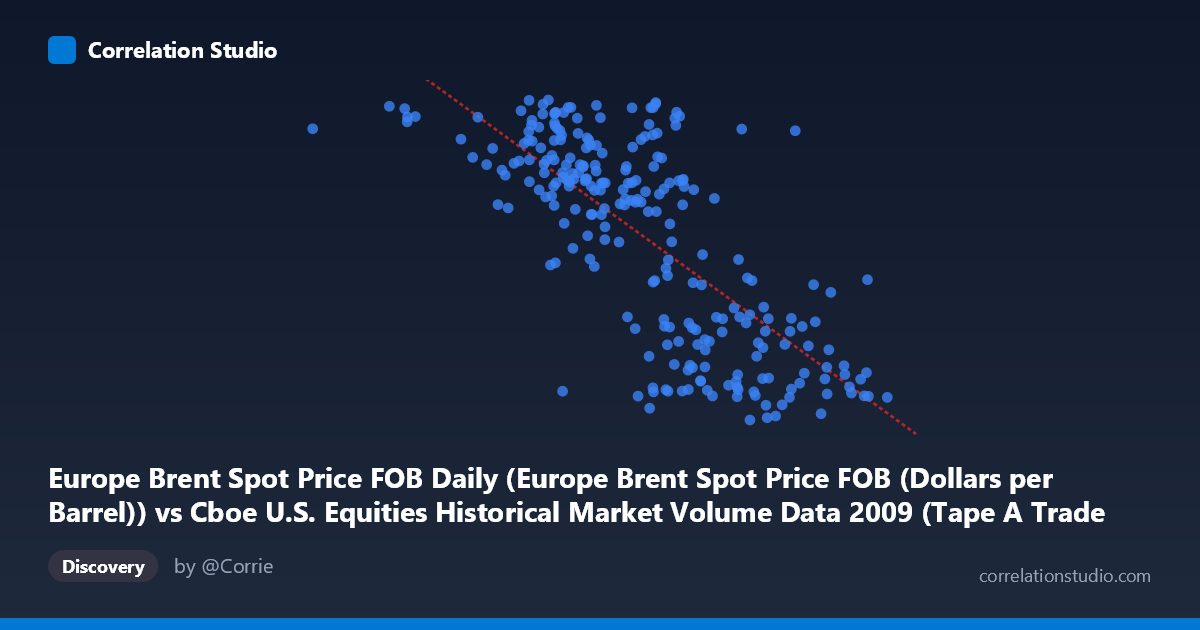
Europe Brent Spot Price FOB Daily (Europe Brent Spot Price FOB (Dollars per Barrel)) vs Cboe U.S. Equities Historical Market Volume Data 2009 (Tape A Trade Count)
- Pearson correlation (r)
- -0.7366
- Spearman correlation
- -0.719
- p-value
- 0
- Sample size (n)
- 252
- 95% confidence interval
- -0.7884 to -0.6744
- Granger causality
- None
- Granger optimal lag
- 1
AI analysis
Scatterplot Analysis: Europe Brent Spot Price vs. U.S. Equities Trade Count (2009)
Relationship Overview
The scatterplot reveals a moderately strong negative relationship between Europe Brent crude oil spot prices (X-axis, in dollars per barrel) and U.S. equities trade counts on Tape A (Y-axis). As oil prices increase, trade counts tend to decrease, and vice versa. The linear regression equation (y = -2.336×10⁻⁵x + 99.80) captures this downward trend, though the scatter around the regression line suggests meaningful variability that the linear model does not fully capture. Visually, data points at lower X values (roughly 362,000–900,000 range on the axis, representing lower oil price periods) cluster at higher Y values, while higher X values correspond to lower trade counts, forming a discernible but imperfect negative slope.
Correlation Strength and Statistical Significance
The Pearson correlation of r = -0.737 indicates a moderately strong negative association, with r² = 0.543 meaning that approximately 54.3% of the variance in Tape A trade counts is explained by Brent crude prices. While this is a meaningful proportion, nearly half the variance remains unexplained, pointing to other influential factors. The 95% confidence interval of [-0.788, -0.674] is relatively tight and does not cross zero, and the p-value is effectively zero, confirming this correlation is highly statistically significant within the 2009 sample (n = 252). However, the Granger causality results are notably inconclusive — neither direction (X→Y: F = 0.258, p = 0.612; Y→X: F = 1.010, p = 0.316) reaches significance at a conventional threshold, meaning that despite a strong contemporaneous correlation, neither variable reliably predicts the other in the next time period. This is a critical caveat: correlation does not imply temporal predictive power here.
Notable Patterns, Clusters, and Outliers
Several structural features stand out in the data. There appears to be a cluster of high trade-count observations (Y values above ~70) concentrated at lower oil price levels, and a separate cluster of lower trade counts (Y ~40–57) at higher oil prices, suggesting a potential bimodal or regime-based structure rather than a smooth linear relationship. One notable outlier is the point at approximately X = 362,081 with Y ≈ 75.15, which represents an extreme low on the X-axis and may correspond to early January 2009 when oil prices were near post-crisis lows. A few points at very high X values (near 2,549,192) also show compressed, low trade counts around 42–44, consistent with late 2009 as oil prices recovered. The spread of residuals appears to widen at intermediate X values, hinting at possible heteroscedasticity.
Confounding Factors and Caveats
The 2009 time period is critical context: this was a year of extraordinary financial market conditions, with the tail of the 2008 financial crisis, a bear market bottom in March, and a significant equity recovery thereafter. Both oil prices and equity trade volumes were heavily influenced by the same macroeconomic shock — fear, deleveraging, and risk appetite — making it highly plausible that a third variable (e.g., macroeconomic uncertainty, VIX, investor risk sentiment) drives both, rather than one causing the other. The axis labels also warrant attention: the X-axis values appear to be scaled in a non-standard way (ranging into the millions for what is nominally a "dollars per barrel" oil price series), suggesting possible unit transformations or dataset merging artifacts that should be verified. Additionally, the N = 3,232 population versus n = 252 sample means the analysis covers only a subset of available data, which could introduce sampling bias depending on selection methodology.
Actionable Insights and Further Investigation
Given the strong contemporaneous correlation but absent Granger causality, the most productive next steps would include: (1) introducing a proxy for macroeconomic risk (e.g., VIX or credit spreads) as a control variable to test whether the correlation is spurious; (2) verifying the X-axis scaling — if oil prices are genuinely in the millions, a unit/data integrity audit is essential before drawing any conclusions; (3) segmenting the data into pre- and post-March 2009 (market trough) to test whether the correlation holds across both regimes or is driven primarily by the crisis period; and (4) applying a non-linear or piecewise regression model to better capture what appears to be threshold behavior visible in the clustering. Any policy or trading conclusions drawn from this correlation alone would be premature given the confounded 2009 environment and the lack of Granger-causal support.
X dataset: Cboe U.S. Equities Historical Market Volume Data 2009
Y dataset: Europe Brent Spot Price FOB Daily
Part of experiment: Daily - Cboe U.S. Equities Historical Market Volume Data 2009 vs Europe Brent Spot Price FOB Daily