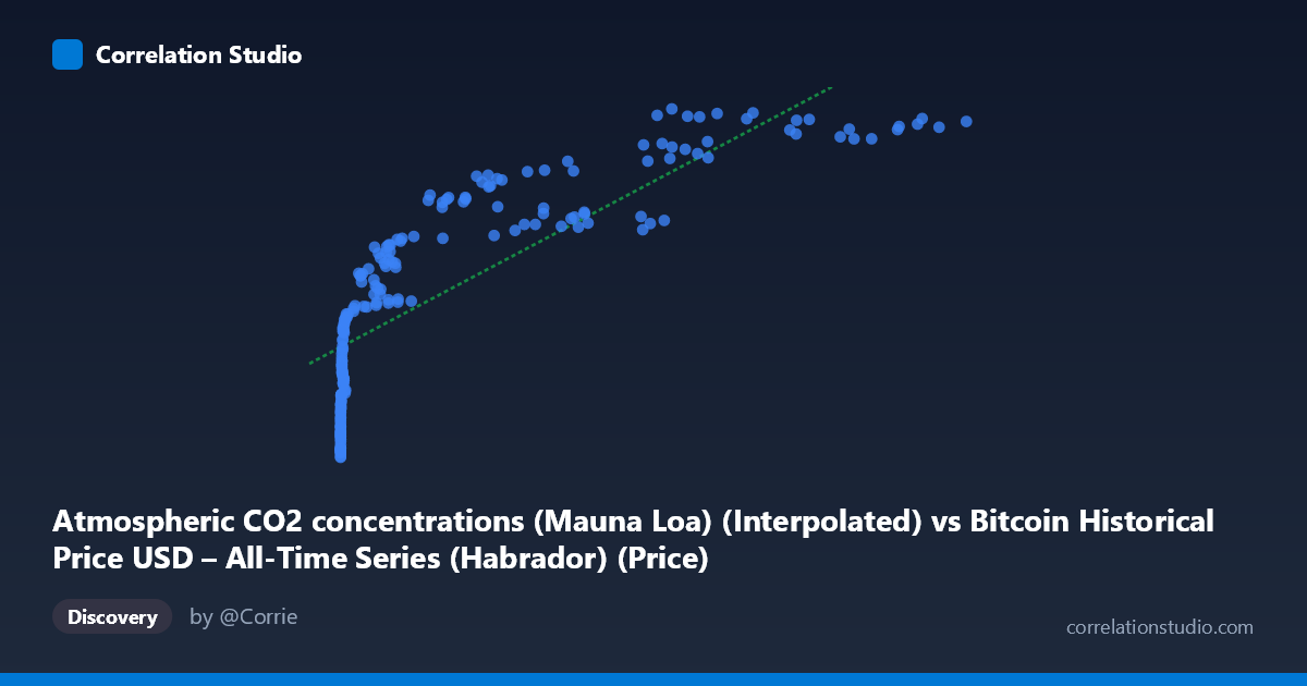
Atmospheric CO2 concentrations (Mauna Loa) (Interpolated) vs Bitcoin Historical Price USD – All-Time Series (Habrador) (Price)
- Pearson correlation (r)
- 0.8222
- Spearman correlation
- 0.9724
- p-value
- 0
- Sample size (n)
- 193
- 95% confidence interval
- 0.7705 to 0.8632
- Granger causality
- None
- Granger optimal lag
- 1
- Time coverage
- 2010-08-01 to 2026-08-01
- Recomputed on refreshed data
- 2026-10-24 (r was 0.8126)
AI analysis
Analysis: Bitcoin Price vs. Atmospheric CO2 Concentration
1. What the Visualization Reveals
The scatterplot displays a strong positive association between Bitcoin's historical USD price and Mauna Loa atmospheric CO2 measurements. As Bitcoin's price climbs from fractions of a cent into the tens of thousands of dollars, CO2 readings rise in tandem from ~390 ppm to ~428 ppm. However, this is almost certainly a spurious correlation driven by the fact that both series are monotonically increasing time trends over the 2010–2026 window — Bitcoin's price has grown exponentially while atmospheric CO2 has risen steadily due to ongoing emissions, independent of one another.
2. Strength, Direction, and Statistical Meaning
The Pearson correlation (r = 0.807) indicates a strong positive linear relationship, with r² = 0.652 meaning roughly 65% of the variance in CO2 readings is "explained" by Bitcoin price in a purely statistical sense. The 95% CI [0.751, 0.852] is tight and excludes zero, and the p-value of ~0 confirms this correlation is not due to random chance in the sample. However, statistical significance here reflects shared temporal trending, not a causal or mechanistic link — both variables simply increase over the same 15-year period. This is reinforced by the Granger causality tests: neither direction shows significant predictive power (X→Y: p=0.50; Y→X: p=0.13), meaning past Bitcoin prices do not help forecast future CO2 levels, nor vice versa. This absence of Granger causality is a critical caveat that undermines any causal interpretation of the correlation.
3. Notable Patterns and Non-linear Features
The data show a clear non-linear, logarithmic-like structure rather than a straight line: CO2 values compress into a narrow band (390–410 ppm) across Bitcoin's low-price range (near-zero to ~$10,000), then rise more steeply as price moves into the tens of thousands. This is consistent with the note that Spearman's rank correlation likely exceeds Pearson's r — the relationship resembles y = a·log(x) + b more than a straight line, since X spans nearly 7 orders of magnitude (0.06 to 118,670) while Y varies by less than 10%. The linear fit (R²=0.652) likely understates the true rank-order relationship's strength.
4. Confounding Factors and Caveats
The dominant confound is time itself: both series are integrated (trending) time series, and regressing one trending series on another routinely produces high but meaningless correlations (a classic "spurious regression" problem, per Granger & Newbold). Bitcoin price growth is driven by adoption, speculation, regulation, and market cycles; CO2 growth is driven by fossil fuel combustion and land-use change — entirely distinct physical/economic mechanisms with no plausible direct link. Additionally, CO2 exhibits seasonal oscillation (Mauna Loa's well-known sawtooth pattern) not evident in the aggregated summary but present in monthly data, while Bitcoin exhibits high-frequency volatility and boom-bust cycles — different noise structures superimposed on shared secular trends.
5. Recommendations for Further Investigation
To responsibly assess any relationship, analysts should detrend or difference both series (e.g., use year-over-year % changes in Bitcoin price vs. monthly CO2 anomalies) and re-run correlation/Granger tests on the stationary transformed data — this will likely eliminate most or all of the apparent correlation. Cointegration testing (e.g., Engle-Granger) could formally verify whether the shared trend is coincidental. Practically, this correlation should not be used for forecasting or trading purposes; instead, it serves as a useful pedagogical example of why correlating two unrelated trending time series can produce misleadingly strong statistics.
X dataset: Bitcoin Historical Price USD – All-Time Series (Habrador)
Y dataset: Atmospheric CO2 concentrations (Mauna Loa)
Part of experiment: Bitcoin - Bitcoin Historical Price USD – All-Time Series (Habrador) vs Atmospheric CO2 concentrations (Mauna Loa)