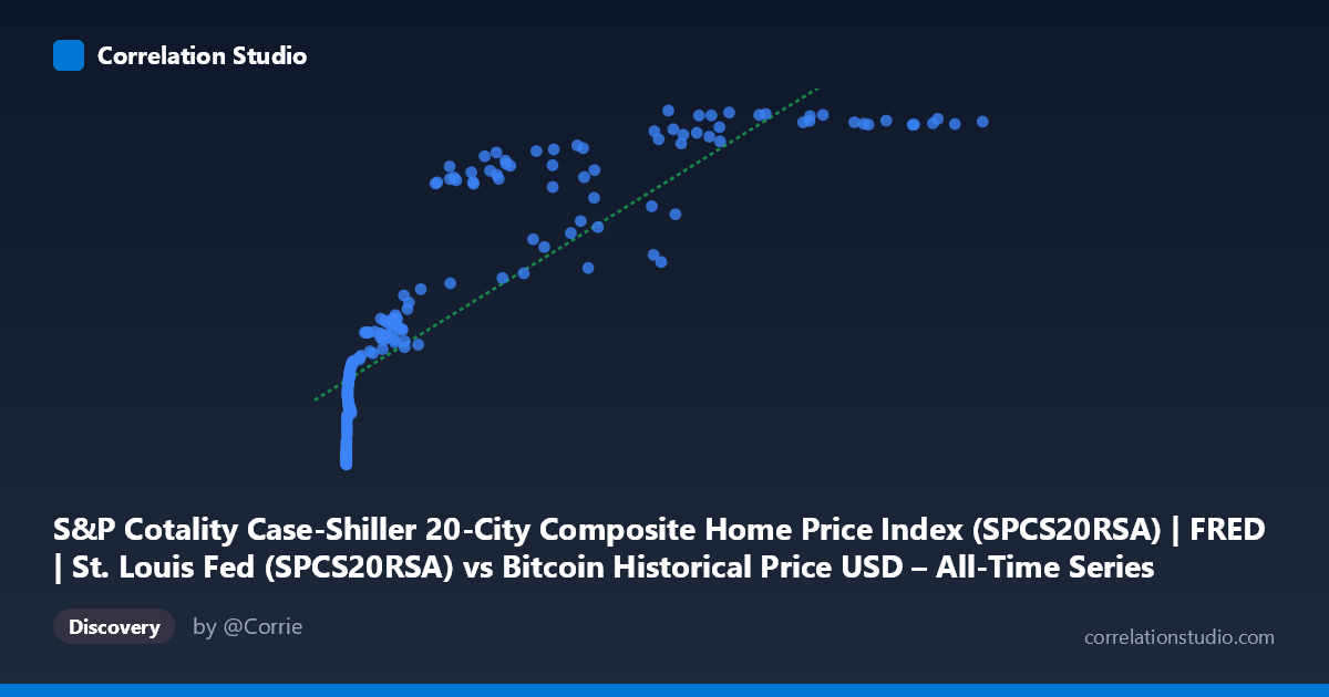
S&P Cotality Case-Shiller 20-City Composite Home Price Index (SPCS20RSA) | FRED | St. Louis Fed (SPCS20RSA) vs Bitcoin Historical Price USD – All-Time Series (Habrador) (Price)
- Pearson correlation (r)
- 0.85
- Spearman correlation
- 0.9702
- p-value
- 0
- Sample size (n)
- 189
- 95% confidence interval
- 0.8049 to 0.8853
- Granger causality
- None
- Granger optimal lag
- 9
AI analysis
Analysis: Bitcoin Price vs. Case-Shiller Home Price Index
1. What the Visualization Reveals
The scatterplot shows a strong positive association between Bitcoin's USD price (X-axis) and the S&P Case-Shiller 20-City Home Price Index (Y-axis). However, the relationship is clearly non-linear: at low Bitcoin prices (under ~$1,000), the Case-Shiller index clusters tightly in the 135–200 range, while as Bitcoin climbs into the tens of thousands, the index rises but with diminishing sensitivity, flattening out near 330–343. This produces a curved, logarithmic-like shape rather than a straight line — consistent with the note that Spearman's rank correlation exceeds Pearson's r, signaling that a log or power-law transformation of X would likely fit the data better than a linear model.
2. Strength, Direction, and Statistical Confidence
The Pearson correlation (r = 0.85) is strong and positive, with r² = 0.7225 indicating that roughly 72% of the variance in the home price index is statistically explained by Bitcoin's price under a linear specification. The 95% CI [0.805, 0.885] is tight and the p-value is effectively zero, meaning the correlation itself is highly statistically robust and not a product of sampling noise. However, statistical significance of correlation should not be confused with causation or predictive utility. The Granger causality tests are decisive on this point: neither direction (Bitcoin→Housing or Housing→Bitcoin) shows significant predictive power (p = 0.61 and p = 0.70, respectively, at the optimal 9-period lag). This means that despite the strong contemporaneous correlation, past values of one series do not meaningfully help forecast future values of the other — the relationship is co-movement, not lead-lag causation.
3. Notable Patterns and Features
Several structural features stand out: - Two-regime clustering: a dense low-X cluster (X < 1,000, Y ≈ 135–220) representing Bitcoin's early years, and a sparser high-X cluster (X 20,000, Y ≈ 250–343) representing recent bull markets. - Ceiling effect in Y: the Case-Shiller index saturates near 335–343 even as Bitcoin ranges from $57,000 to $118,000, suggesting the housing index has its own independent growth ceiling/trend unrelated to Bitcoin's continued volatility. - Non-monotonic wiggles: at high X, Y occasionally dips (e.g., X=45,092 → Y=252.72 and X=56,973 → Y=289.15) amid neighboring higher-Y points, reflecting Bitcoin's own boom-bust cycles that don't map cleanly onto the steadily rising housing index. - Extreme X-range skew: X spans nearly 6 orders of magnitude (0.06 to 118,670) while Y spans a much narrower range (136 to 343), which naturally produces curvature and log-linear-style compression on a raw linear scale.
4. Confounding Factors and Caveats
This correlation is almost certainly driven by a shared time trend rather than any direct economic mechanism. Both series have risen substantially over 2010–2026 as part of broader macro trends (monetary expansion, low interest rates, inflation, retail investment growth). Time itself is a lurking confounder: any two upward-trending time series will show spurious correlation regardless of true causal linkage. The lack of Granger causality reinforces this — it's consistent with two independent trending series rather than a genuine causal interaction. Additionally, Bitcoin's data likely has daily/high-frequency granularity while Case-Shiller is a monthly, smoothed, lagged index, creating a temporal mismatch and effective autocorrelation that inflates apparent correlation strength.
5. Suggested Next Steps
To move beyond this potentially spurious linear correlation, analysts should: (1) detrend or difference both series (e.g., use year-over-year % change instead of levels) and recompute correlation — trending-series correlations often collapse once trends are removed; (2) fit a log-linear or log-log model given the Spearman/Pearson divergence, since log(Bitcoin price) may correlate more linearly with the index; (3) test cointegration (e.g., Engle-Granger) rather than simple correlation, which is more appropriate for two potentially non-stationary trending series; and (4) introduce macro control variables (interest rates, CPI, M2 money supply) to check whether the apparent relationship is fully mediated by shared macroeconomic drivers rather than any direct link between crypto and housing markets.
X dataset: Bitcoin Historical Price USD – All-Time Series (Habrador)
Y dataset: S&P Cotality Case-Shiller 20-City Composite Home Price Index (SPCS20RSA) | FRED | St. Louis Fed
Part of experiment: Bitcoin - Bitcoin Historical Price USD – All-Time Series (Habrador) vs S&P Cotality Case-Shiller 20-City Composite Home Price Index (SPCS20RSA) | FRED | St. Louis Fed