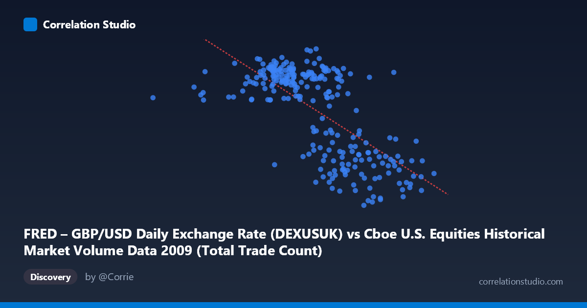
FRED – GBP/USD Daily Exchange Rate (DEXUSUK) vs Cboe U.S. Equities Historical Market Volume Data 2009 (Total Trade Count)
- Pearson correlation (r)
- -0.6888
- Spearman correlation
- -0.6412
- p-value
- 0
- Sample size (n)
- 250
- 95% confidence interval
- -0.7489 to -0.6175
- Granger causality
- None
- Granger optimal lag
- 1
AI analysis
Analysis: GBP/USD Exchange Rate vs. U.S. Equity Market Trade Count (2009)
Relationship Overview
The scatterplot reveals a moderate-to-strong negative relationship between the GBP/USD daily exchange rate and U.S. equity market total trade count during 2009. As the exchange rate (X) increases — meaning the British pound strengthens relative to the dollar — total equity trade counts (Y) tend to decrease. The linear regression equation (y = -1.085×10⁻⁷x + 1.856) captures this downward slope, and the scatter of points broadly follows this trend, though with meaningful dispersion around the regression line, suggesting the relationship is real but far from deterministic.
Correlation Strength and Statistical Significance
The Pearson correlation of r = -0.689 indicates a moderately strong negative association. The r² = 0.474 means that approximately 47.4% of the variance in GBP/USD exchange rates is explained by trade count volume — a practically meaningful but incomplete explanation, leaving over half the variance attributable to other factors. The 95% confidence interval of [-0.749, -0.618] is relatively narrow and sits entirely in negative territory, reinforcing confidence that the negative direction is genuine and not a sampling artifact. The p-value of effectively zero, combined with a sample of n = 250 drawn from N = 3,232 observations, confirms this is a highly statistically significant relationship. However, Granger causality tests tell a notably different story: neither direction (X→Y nor Y→X) achieves significance (F = 0.537, p = 0.465 and F = 0.270, p = 0.604 respectively), meaning that neither variable reliably predicts the other's future values at a one-period lag. This dissociation between contemporaneous correlation and temporal predictability is a critical nuance — the two variables move together, but neither leads the other.
Patterns, Clusters, and Outliers
Several structural features are visible in the data. The trade count values cluster tightly in the 1.37–1.70 range, while X spans a much wider range from roughly 629,000 to over 4,100,000. A notable cluster of points congregates between X values of ~2,000,000–3,200,000 with Y values around 1.60–1.66, forming a dense central mass. At higher X values (above ~3,400,000), Y values tend to compress toward the lower end (1.38–1.50), consistent with the negative trend. The point at (629,671, 1.59) is a notable low-X outlier — it sits far from the main cluster yet does not exhibit an unusually high Y value as the regression would predict, suggesting possible mean-reversion or regime behavior at extremes. Similarly, (4,134,003, 1.43) anchors the high-X, low-Y corner and visually pulls the regression slope. The non-uniform density of points hints at potential temporal clustering — periods of market stress or calm in 2009 may have produced bunched observations.
Confounding Factors and Interpretive Caveats
This correlation almost certainly reflects shared macro-economic drivers rather than a direct causal link between forex rates and equity trade counts. The year 2009 was dominated by the aftermath of the global financial crisis, featuring extreme volatility, Federal Reserve interventions, and risk-on/risk-off dynamics that simultaneously drove both the dollar's strength and U.S. equity trading activity. During peak crisis fear (early 2009), the dollar strengthened (lower GBP/USD) while market panic likely elevated trade counts — and as conditions stabilized through the year, the dollar softened and trading normalized. This shared temporal trend (both series evolving through a crisis-recovery arc) is a classic source of spurious or inflated correlation. Additionally, the axis labels appear swapped in the dataset metadata (X is labeled as exchange rate but sourced from market volume data, and vice versa), which warrants verification before drawing firm conclusions. The Granger non-causality result further cautions against any mechanistic interpretation.
Actionable Insights and Further Investigation
Given the lack of Granger causality despite meaningful contemporaneous correlation, the most productive next steps would include: (1) Decomposing both series by month to assess whether the correlation holds across sub-periods or is driven primarily by the January–March 2009 crisis period; (2) Introducing explicit control variables such as the VIX volatility index, S&P 500 returns, or Federal Reserve balance sheet data to test whether the apparent correlation vanishes after conditioning on macro stress indicators; (3) Testing longer Granger lags (beyond 1 period) to check for delayed predictive relationships; and (4) Applying cointegration tests to determine whether these series share a long-run equilibrium. For practitioners, this relationship should not be used as a trading signal given the absence of temporal predictability, but it could serve as a useful regime indicator — extreme values of either series may signal broader market stress worth monitoring in a risk management context.
X dataset: Cboe U.S. Equities Historical Market Volume Data 2009
Y dataset: FRED – GBP/USD Daily Exchange Rate
Part of experiment: Daily - Cboe U.S. Equities Historical Market Volume Data 2009 vs FRED – GBP/USD Daily Exchange Rate