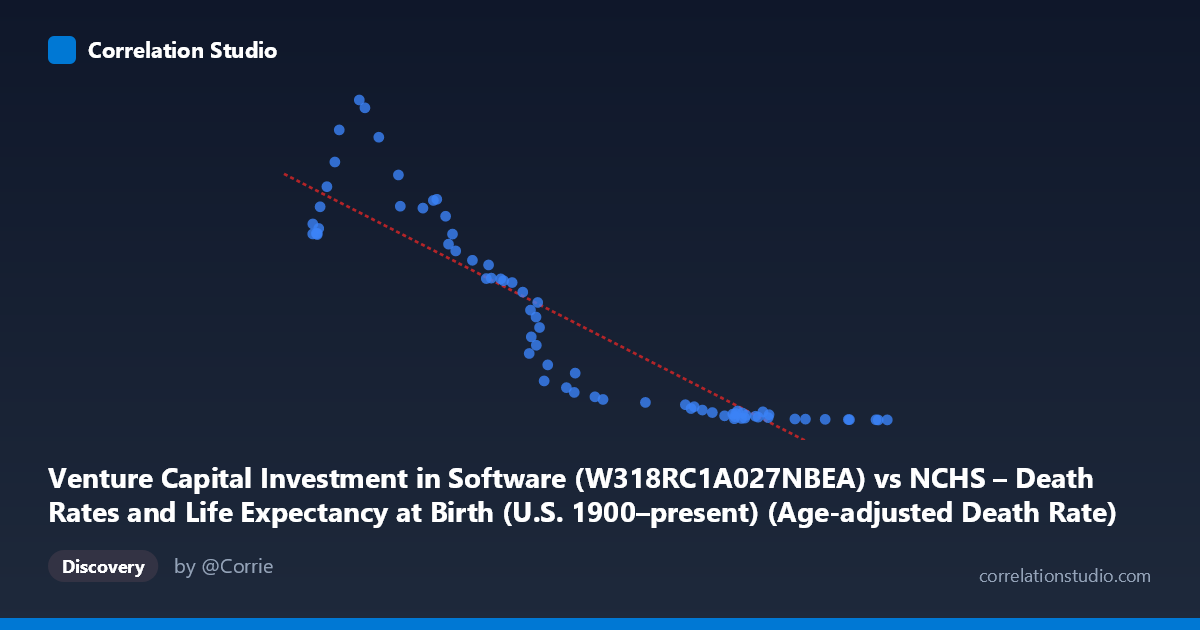
Venture Capital Investment in Software (W318RC1A027NBEA) vs NCHS – Death Rates and Life Expectancy at Birth (U.S. 1900–present) (Age-adjusted Death Rate)
- Pearson correlation (r)
- -0.9076
- Spearman correlation
- -0.962
- p-value
- 0
- Sample size (n)
- 73
- 95% confidence interval
- -0.9411 to -0.8563
- Granger causality
- None
- Granger optimal lag
- 10
- Time coverage
- 1946-01-01 to 2018-01-01
AI analysis
Analysis: Venture Capital Software Investment vs. Age-Adjusted Death Rate
1. Overall Relationship
The scatterplot reveals a strong negative relationship between U.S. venture capital investment in software and the age-adjusted death rate. As software investment has grown — ranging from roughly $777B to $1,599B — the death rate has fallen dramatically, from a high near 466 per 100,000 down to values below 5. The linear regression equation (y = −0.520x + 741.6) captures this inverse trend reasonably well across most of the observed range, though the scatter suggests the true relationship may be nonlinear, particularly at the extremes of the X distribution.
2. Correlation Strength and Statistical Framing
The Pearson correlation of r = −0.908 indicates a very strong negative association, and the R² of 0.824 means that roughly 82% of the variance in age-adjusted death rates is statistically "explained" by variation in software investment levels. The 95% confidence interval [−0.941, −0.856] is narrow and entirely negative, confirming the direction is not a sampling artifact, and the p-value of effectively zero reinforces that this association is highly unlikely under a null hypothesis of no relationship. However, the Granger causality results are a critical corrective: neither direction (X→Y nor Y→X) achieves statistical significance (F ≈ 0.67, p ≈ 0.75 for X→Y; F ≈ 0.60, p ≈ 0.80 for Y→X at lag 10). This means that, despite the impressive correlation, past values of software investment do not meaningfully predict future death rates, and vice versa — a strong warning against any causal narrative.
3. Notable Patterns, Clusters, and Outliers
Several structural features stand out in the data. There is a dense cluster in the upper-left region (X ≈ 776–900, Y ≈ 270–466), corresponding to earlier time periods with lower investment and higher mortality, and a compressed cluster in the lower-right (X ≈ 1,400–1,600, Y ≈ 1–15), representing recent years with high investment and very low death rates. The relationship appears visibly nonlinear — the rate of decline in Y is steep at lower X values but flattens dramatically as X exceeds ~1,200, suggesting a potential exponential or power-law decay rather than a simple linear form. Points like (843, 466) and (851, 455) represent notable high-mortality observations, while (1,586–1,599, <1) represent the extreme low-mortality, high-investment end. The linear model likely understates Y at mid-range X values and overstates it at the extremes.
4. Confounding Factors and Caveats
This correlation is a textbook example of spurious correlation driven by shared secular time trends. Both variables are strongly time-dependent: software investment has grown consistently due to technological and economic expansion since the mid-20th century, while age-adjusted death rates have declined steadily due to advances in medicine, public health infrastructure, improved nutrition, reduced smoking rates, and better chronic disease management. Any two variables that trend in opposite directions over the same decades will correlate strongly — the 1946–2018 time span virtually guarantees this overlap. Furthermore, the dataset labels appear internally inconsistent (the X-axis column is labeled as coming from a death rates dataset, and vice versa), raising data provenance questions. The optimal Granger lag of 10 periods is quite long and may obscure meaningful shorter-term dynamics, or simply reflect the absence of any true predictive mechanism.
5. Actionable Insights and Further Investigation
The most important takeaway is that this correlation should not be interpreted causally in either direction. Software investment does not reduce mortality, and declining death rates do not drive tech investment — both are downstream of broader socioeconomic modernization. For further investigation, researchers should: (1) detrend both time series (e.g., via first-differencing or HP filtering) before computing correlations to remove the shared secular trend; (2) test nonlinear model fits (logarithmic or exponential decay) given the apparent curvature in the scatterplot; (3) introduce explicit confounders such as GDP per capita, healthcare expenditure, or population age structure to partial out shared drivers; and (4) verify dataset column assignments, as the axis labels suggest a possible data swap that could affect interpretability. The real analytical value here may lie in using this as a pedagogical case study in distinguishing correlation from causation in long-run time series data.
X dataset: NCHS – Death Rates and Life Expectancy at Birth (U.S. 1900–present)
Y dataset: Venture Capital Investment in Software
Part of experiment: Yearly - NCHS – Death Rates and Life Expectancy at Birth (U.S. 1900–present) vs Venture Capital Investment in Software