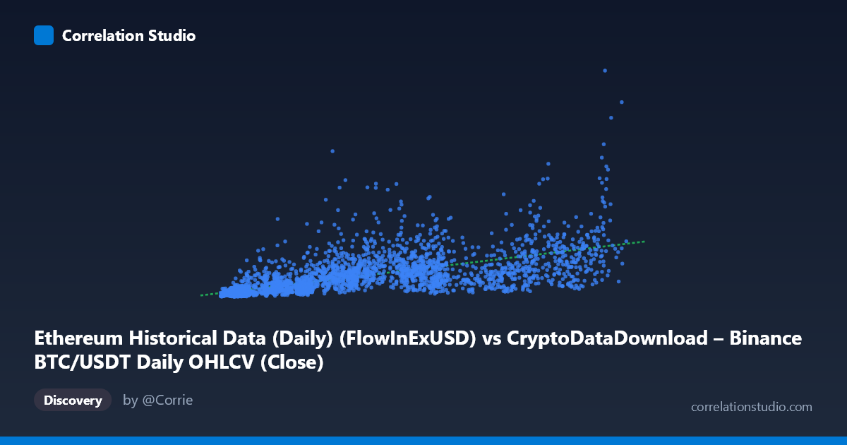
Ethereum Historical Data (Daily) (FlowInExUSD) vs CryptoDataDownload – Binance BTC/USDT Daily OHLCV (Close)

Pearson correlation (r): 0.6562
Spearman correlation: 0.8171
p-value: 0
Sample size (n): 3191
95% confidence interval: 0.636 to 0.6755
Granger causality: Y → X
Granger optimal lag: 10

AI analysis

Analysis of the Relationship Between X and Y Variables

1. What the Visualization Reveals

The scatterplot depicts a positive, moderately strong association between the X variable (labeled as ETH flow-in, though the values and scale suggest this may actually be mislabeled metadata) and the Y variable (labeled as BTC/USDT close price, again likely a metadata mismatch given the billions-scale magnitude). Regardless of labeling ambiguity, the data show that as X increases, Y tends to increase as well, but with substantial scatter — particularly at low-to-mid X values, where Y ranges from ~50 million to over 1.5 billion for X values clustered between 4,000–30,000. This spread narrows somewhat at higher X values (80,000), where Y values tend to stabilize in a lower, tighter band relative to the extreme peaks seen at moderate X.

2. Strength, Direction, and Statistical Confidence

The Pearson correlation (r = 0.656) indicates a moderate-to-strong positive linear relationship, with r² = 0.431 meaning only 43% of the variance in Y is explained by X — leaving the majority (57%) attributable to other factors, noise, or non-linear dynamics not captured by this simple linear framing. The 95% confidence interval [0.636, 0.676] is tight given the large sample size (n=3,191), and the p-value of ~0 confirms the correlation is highly statistically significant and not due to chance. However, statistical significance with large n is expected even for modest effect sizes — practical significance is better judged by r² here, which suggests a real but incomplete explanatory relationship.

The Granger causality results add an important temporal dimension: Y Granger-causes X (F=2.64, p=0.0033) at an optimal lag of 10 periods, while X does not significantly Granger-cause Y (p=0.146). This suggests that past values of Y have predictive power for future X, but not vice versa — implying Y may be a leading indicator or driver in this system, contrary to what a naïve reading of "X predicts Y" from the regression equation might imply. This is a critical distinction: correlation/regression describes covariation, but Granger causality describes temporal precedence.

3. Notable Patterns and Non-Linear Features

Several data points stand out as high-leverage outliers: for instance, X≈36,445 pairs with Y≈1.57 billion, and X≈78,596 with Y≈1.53 billion — both far above the regression line's predicted value (~12,385×X + 87.3M ≈ 450M–970M range). These spikes at low-to-mid X values pull the linear fit's slope down and inflate residual variance. The note that Spearman's ρ exceeds Pearson's r is a strong signal that the relationship is monotonic but non-linear — likely logarithmic or power-law in shape, consistent with typical financial/crypto data where growth compounds or volatility scales multiplicatively rather than additively. A log-transform of Y (or both variables) would likely tighten the fit considerably and better represent the true relationship.

4. Confounding Factors and Caveats

Given the metadata, both variables are derived from cryptocurrency market data over 2017–2026, a period marked by extreme bull/bear cycles, halving events, regulatory shocks, and macro liquidity conditions (e.g., Fed rate changes). Both BTC and ETH prices/flows are highly correlated with overall crypto market sentiment and Bitcoin dominance cycles — meaning this relationship is likely confounded by a shared latent factor (broad market risk appetite) rather than direct causal linkage between the two specific metrics. Additionally, if X and Y labels are indeed swapped or mismatched (as the described columns suggest — "FlowInExUSD" vs. "Close" price — yet the scales don't clearly align with typical ETH exchange flow figures), any causal or economic interpretation should be treated cautiously until the schema is verified.

5. Actionable Insights and Further Investigation

1. Re-run regression using log(Y) or log(X)-log(Y) transforms to test the non-linear hypothesis suggested by the Spearman/Pearson divergence — this should improve R² substantially. 2. Investigate the outlier cluster (X: 30k–80k, Y 1.4B) — these may correspond to specific volatile market events (e.g., 2021 bull run, 2024 halving rally) and warrant a time-series overlay to check for temporal clustering. 3. Leverage the Granger causality finding: build a lagged predictive model using Y(t-1...t-10) to forecast X(t), rather than assuming X drives Y — this reverses the naive regression narrative and could inform trading/allocation strategies. 4. Verify column/schema alignment given the unusual axis label descriptions — mismatched or mislabeled data would invalidate domain-specific conclusions (e.g., "ETH flow drives BTC price" vs. the reverse). 5. Control for time/market regime (bull vs. bear phases) via a multivariate or regime-switching model to isolate whether the X-Y relationship is stable or regime-dependent, given the multi-year span covering several major crypto cycles.

X dataset: CryptoDataDownload – Binance BTC/USDT Daily OHLCV

Y dataset: Ethereum Historical Data (Daily)

Part of experiment: Bitcoin - CryptoDataDownload – Binance BTC/USDT Daily OHLCV vs Ethereum Historical Data (Daily)