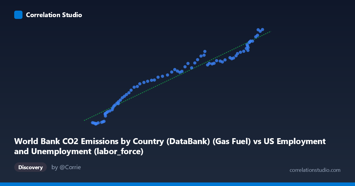
World Bank CO2 Emissions by Country (DataBank) (Gas Fuel) vs US Employment and Unemployment (labor_force)
- Pearson correlation (r)
- 0.9744
- Spearman correlation
- 0.9895
- p-value
- 0
- Sample size (n)
- 80
- 95% confidence interval
- 0.9603 to 0.9836
- Granger causality
- None
- Granger optimal lag
- 10
AI analysis
Scatterplot Analysis: US Gas Fuel CO2 Emissions vs. US Labor Force
Relationship Overview
The scatterplot reveals a remarkably strong, positive, and nearly linear relationship between US gas fuel CO2 emissions (X-axis) and the US labor force size (Y-axis) spanning eight decades from 1941 to 2020. As gas fuel emissions increase from roughly 53,860 to 163,539 (thousand metric tons), the labor force grows correspondingly from approximately 654 to 16,992 (thousands). The data points cluster tightly around the regression line y = 0.128x − 4,945.56, suggesting that both variables have grown in near-lockstep over this long historical period. This co-movement reflects the shared underlying driver of broad economic and demographic expansion rather than any direct mechanistic link between gas combustion and workforce size.
Correlation Strength and Statistical Significance
The correlation is exceptionally strong at r = 0.9744, and the coefficient of determination r² = 0.9495 indicates that approximately 94.9% of the variance in labor force size is statistically explained by variation in gas fuel CO2 emissions within this sample. The 95% confidence interval of [0.9603, 0.9836] is narrow and entirely in the high-positive range, confirming that this is a robust and precisely estimated association rather than a sampling artifact. The p-value of effectively 0 (against N = 86, n = 80 paired observations) means the probability of observing a correlation this strong by chance under the null hypothesis of no relationship is vanishingly small. However, despite this statistical power, the Granger causality analysis returns no significant predictive direction in either direction (X→Y: F = 1.18, p = 0.33; Y→X: F = 0.86, p = 0.58) at the optimal lag of 10 periods. This is a critical finding: neither variable meaningfully predicts the future changes in the other once their shared trend is accounted for, strongly suggesting that the observed correlation is driven by a common underlying trend rather than any causal pathway between them.
Notable Patterns, Clusters, and Outliers
The data display a clear two-regime structure when examined closely. The lower-left cluster (X: ~53,000–75,000; Y: ~654–5,500) corresponds to earlier decades (1940s–1960s), where both emissions and labor force were comparatively modest and data points are more densely packed with slightly higher scatter relative to the trend line. The upper-right cluster (X: ~130,000–163,500; Y: ~11,000–16,992) represents recent decades with both variables at their peaks and notably tight adherence to the regression line. The transition zone in the middle range shows smooth, continuous progression with minimal deviation. There are no dramatic outliers, though a handful of points in the lower-left region (e.g., the point near X = 55,910, Y = 654 and X = 53,860, Y = 877) sit slightly below the regression line, potentially reflecting early wartime labor force disruptions or measurement differences in the earliest years of coverage.
Confounding Factors and Interpretive Caveats
The near-perfect correlation almost certainly reflects spurious co-trending rather than a genuine causal relationship. Both gas fuel CO2 emissions and labor force size are fundamentally driven by population growth, GDP expansion, industrialization, and energy demand — all of which trend upward together over an 80-year horizon. This is a textbook case of what econometricians call a spurious regression between non-stationary time series: when two variables share a common upward trend, their correlation will be artificially inflated regardless of whether they are causally connected. The Granger causality results reinforce this interpretation. Additional caveats include: (1) the X-axis dataset is labeled as originating from an employment dataset, which raises potential data provenance concerns worth verifying; (2) the linear model may mask structural breaks such as the 1970s oil shocks, the 2008–2009 financial crisis, or the COVID-19 disruption in 2020; and (3) aggregating to annual national-level data obscures sectoral, regional, and demographic heterogeneity.
Actionable Insights and Further Investigation
Given the spurious co-trending concern, the most important next analytical step is to first-difference or detrend both series (e.g., using year-over-year growth rates) and re-examine whether any meaningful correlation persists after removing the shared trend component. A cointegration test (e.g., Engle-Granger or Johansen) would help determine whether these series share a statistically valid long-run equilibrium relationship beyond mere parallel trending. Researchers should also control for GDP or population as explicit covariates to isolate whether gas emissions carry independent explanatory power for labor force dynamics. More substantively, it would be valuable to disaggregate emissions by sector (transportation, industrial, residential) and correlate those against specific labor market categories (manufacturing employment, service employment) to test whether any segment-level relationships are more causally plausible. Finally, introducing structural break analysis around key economic shocks would clarify whether the linear relationship holds uniformly or masks important regime changes across this 80-year period.
X dataset: US Employment and Unemployment
Y dataset: World Bank CO2 Emissions by Country (DataBank)
Part of experiment: Yearly - US Employment and Unemployment vs World Bank CO2 Emissions by Country (DataBank)