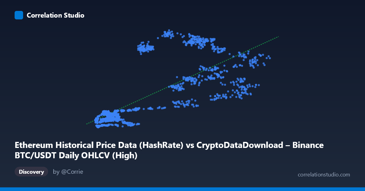
Ethereum Historical Price Data (HashRate) vs CryptoDataDownload – Binance BTC/USDT Daily OHLCV (High)
- Pearson correlation (r)
- 0.7484
- Spearman correlation
- 0.7526
- p-value
- 0
- Sample size (n)
- 1855
- 95% confidence interval
- 0.7277 to 0.7678
- Granger causality
- None
- Granger optimal lag
- 1
- Time coverage
- 2017-08-17 to 2022-09-14
AI analysis
Analysis: Relationship Between Ethereum Hash Rate Metric (X) and BTC/USDT High Price (Y)
Note on labeling: The axis labels appear swapped or mismatched in the metadata (X is labeled "Ethereum Historical Price Data (HashRate)" but the dataset description is BTC/USDT OHLCV, while Y is explicitly BTC/USDT High). Given the value ranges (X: 3,276–69,000; Y: 83–1,065), this is more consistent with X representing a Bitcoin-related price/volume metric and Y representing Ethereum's daily high price, or both being price series from correlated crypto markets. The analysis below treats X and Y as given, but this labeling ambiguity should be resolved before drawing asset-specific conclusions.
1. What the Visualization Reveals
The scatterplot shows a clear positive, moderately strong association: as X increases, Y tends to increase as well. The relationship is not perfectly linear — there's noticeable heteroscedasticity, with tight clustering at low X values (roughly 3,000–15,000) where Y stays compressed between 100–250, and much wider vertical spread at higher X values (20,000–60,000) where Y ranges anywhere from ~270 to over 1,000. This fan-shaped pattern suggests the linear model captures the broad trend but misses regime-dependent behavior.
2. Strength, Direction, and Statistical Confidence
The correlation coefficient (r = 0.7484, R² = 0.560) indicates a strong positive relationship, with the linear model explaining 56% of the variance in Y. The remaining 44% is driven by other factors — plausibly market-specific dynamics, volatility clustering, or regime shifts (bull/bear cycles) not captured by a simple linear fit with X alone. The 95% CI [0.728, 0.768] is tight and the p-value is effectively 0, meaning we can be highly confident this correlation is real and not a sampling artifact — with n=1,855 paired observations, statistical power is high.
However, correlation here should not imply causation or predictive utility in a trading sense. The Granger causality tests show no significant predictive direction in either direction (X→Y: p=0.306; Y→X: p=0.460). This is a critical finding: despite the strong contemporaneous correlation, past values of X do not help forecast future Y, nor vice versa, at a 1-period lag. This pattern is classic for two variables that are both driven by a common underlying factor (e.g., overall crypto market sentiment, macro liquidity conditions, or shared exchange/network activity) rather than one causing the other.
3. Notable Patterns and Outliers
Several data points break the linear trend and warrant attention: - High-Y, moderate-X outliers: e.g., (20792, 939.71), (21348, 873.68), (30488, 1016.21) — these points sit far above the regression line, suggesting periods where Y spiked disproportionately relative to X (possibly a market euphoria/bubble phase). - Low-Y, high-X outliers: e.g., (56100, 715.06) sits below what similar X values elsewhere suggest, and points like (17720, 110.65) and (11190, 110.03) fall well below the low-X cluster, indicating temporal regime effects rather than a smooth functional relationship. - The data appears to split into at least two "clusters" or regimes: a low-X/low-Y baseline period and a high-X/high-Y period with much greater dispersion — consistent with distinct market cycles (e.g., 2020–2021 bull run vs. 2018–2019 bear market) rather than a single stable relationship holding throughout.
4. Confounding Factors and Caveats
- Time-series autocorrelation: Both variables are financial time series and likely non-stationary (trending), which can inflate correlation coefficients due to shared trends rather than genuine coupling. Standard Pearson r on trending series often overstates the "true" relationship. - Common market driver: Crypto assets are notoriously correlated due to shared macro factors (BTC dominance effects, overall risk appetite, USD liquidity, regulatory news) — the correlation may reflect this systemic co-movement rather than a direct mechanical link between the two specific variables. - Label ambiguity: As noted, the metadata's mismatched column descriptions make it unclear exactly what X represents, which limits confident domain interpretation. - Non-stationarity affects Granger test validity: If either series has a unit root, Granger causality results can be unreliable unless the data was differenced/detrended first — this should be verified.
5. Suggestions for Further Investigation
1. Clarify data provenance — confirm what X actually measures before drawing further conclusions. 2. Detrend or difference both series (e.g., use daily returns instead of levels) and re-run correlation and Granger tests to check if the relationship holds for changes rather than levels — this is standard practice in financial time-series analysis and would give a cleaner causal picture. 3. Segment by time period/regime (bull vs. bear market) to test whether the relationship strength and slope are stable or regime-dependent, given the fan-shaped dispersion pattern observed. 4. Test a log-log or nonlinear model given the multiplicative nature of price data and the increasing variance at higher X — this may improve fit and explain more of the currently-unexplained 44% variance. 5. Investigate the identified outlier periods directly to understand what news/market events drove the divergence from the linear trend during those windows.
X dataset: CryptoDataDownload – Binance BTC/USDT Daily OHLCV
Y dataset: Ethereum Historical Price Data
Part of experiment: Bitcoin - CryptoDataDownload – Binance BTC/USDT Daily OHLCV vs Ethereum Historical Price Data