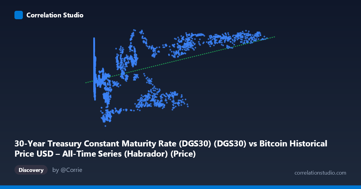
30-Year Treasury Constant Maturity Rate (DGS30) (DGS30) vs Bitcoin Historical Price USD – All-Time Series (Habrador) (Price)
- Pearson correlation (r)
- 0.478
- Spearman correlation
- 0.1495
- p-value
- 0
- Sample size (n)
- 3946
- 95% confidence interval
- 0.4536 to 0.5017
- Granger causality
- None
- Granger optimal lag
- 1
AI analysis
Analysis: Bitcoin Price vs. 30-Year Treasury Yield
1. What the Visualization Reveals
Note first that the axis labels appear swapped in the metadata — the actual data shows X as Bitcoin price (range 0.05 to 124,720, consistent with BTC's historical USD range) and Y as the 30-Year Treasury yield (range 0.99% to 5.11%, consistent with historical DGS30 values). Interpreting the data this way: the scatterplot shows a weak-to-moderate positive relationship where higher Bitcoin prices tend to coincide with higher long-term Treasury yields. At low Bitcoin prices (under $1,000), yields scatter broadly between roughly 2.2% and 4.5%, while at high Bitcoin prices (above $60,000), yields cluster more consistently in the 4.0–5.0% range, suggesting the relationship strengthens or becomes less noisy at the extremes.
2. Strength, Direction, and Statistical Confidence
The correlation coefficient (r = 0.478) indicates a weak-to-moderate positive relationship. Critically, r² = 0.229 means only about 23% of the variance in one variable is explained by the other — roughly 77% of the movement is driven by other factors entirely. The 95% CI [0.454, 0.502] is fairly tight given the large sample (n=3,946), and the p-value of ~0 confirms this correlation is statistically significant and not due to chance. However, statistical significance here reflects sample size, not practical strength — with thousands of data points, even modest correlations become "significant." The Granger causality tests are the most important caveat: neither direction shows significant predictive power (X→Y: p=0.134; Y→X: p=0.191). This means neither Bitcoin price nor Treasury yields reliably help forecast the other's future values — the correlation is likely coincidental co-movement (e.g., both trending upward over 2010–2026) rather than a causal or predictive mechanism.
3. Notable Patterns and Outliers
The data reveals a time-trend confound: both series have risen dramatically over the sample period (2010–2026). Bitcoin went from fractions of a cent to over $100,000; 30-year yields drifted from historic lows (~1-2%, post-2008 crisis era) to higher levels (~4.5-5%, reflecting 2022-2024 rate hikes). This produces a spurious-looking correlation driven by shared temporal trends rather than genuine interaction. Notable clusters include a dense low-X/low-to-mid-Y region (early Bitcoin history, 2010-2016) and a sparser high-X cluster (2020s bull runs) where yields are elevated. Some outliers exist — e.g., a Bitcoin price near $57,000 paired with a yield of only 1.77%, and $34,575 paired with 1.93% — showing periods of high BTC price coinciding with low yields (likely 2020-2021 pandemic-era near-zero rate environment), which break the general positive trend.
4. Confounding Factors and Caveats
The most significant confound is time itself: both variables are trending series over a 16-year span, and non-stationary trending data frequently produces inflated correlations that don't reflect genuine relationships (a classic "spurious regression" problem). Macroeconomic regimes — quantitative easing (2010-2015, 2020-2021), inflation surges (2022-2023), and Fed rate hiking cycles — independently affected both crypto speculation and bond yields without one causing the other. Bitcoin's price is influenced by adoption cycles, halving events, and speculative bubbles, while 30-year yields respond to inflation expectations, Fed policy, and fiscal conditions — these are largely independent causal systems that happen to share a macro backdrop of "post-2008 to post-pandemic monetary normalization."
5. Recommendations for Further Investigation
Given the non-stationarity concern, analysts should difference or detrend both series (e.g., using returns/changes rather than levels) and re-run correlation and Granger tests — this is standard practice to avoid spurious correlation in trending time series. Testing for cointegration (e.g., Engle-Granger or Johansen tests) would clarify whether there's a genuine long-run equilibrium relationship. Segmenting the analysis by distinct monetary policy regimes (ZIRP era vs. hiking cycles) may reveal whether the relationship is regime-dependent rather than constant. Finally, given the failed Granger causality results, this correlation should not be used for predictive trading strategies linking rates to crypto prices — instead, treat both as responding to a common set of macro drivers (inflation, liquidity, risk sentiment) worth modeling directly.
X dataset: Bitcoin Historical Price USD – All-Time Series (Habrador)
Y dataset: 30-Year Treasury Constant Maturity Rate (DGS30)
Part of experiment: Bitcoin - Bitcoin Historical Price USD – All-Time Series (Habrador) vs 30-Year Treasury Constant Maturity Rate (DGS30)