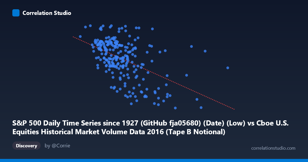
S&P 500 Daily Time Series since 1927 (GitHub fja05680) (Date) (Low) vs Cboe U.S. Equities Historical Market Volume Data 2016 (Tape B Notional)
- Pearson correlation (r)
- -0.5097
- Spearman correlation
- -0.4948
- p-value
- 0
- Sample size (n)
- 252
- 95% confidence interval
- -0.5958 to -0.4121
- Granger causality
- None
- Granger optimal lag
- 1
AI analysis
Scatterplot Analysis: S&P 500 Daily Low vs. Cboe Tape B Notional Volume (2016)
1. Overall Relationship
The scatterplot reveals a moderate negative relationship between the S&P 500 daily low price and Cboe Tape B notional trading volume for 2016. As the S&P 500 daily low increases (i.e., markets trade at higher price levels), Tape B notional volume tends to decrease. This inverse pattern is broadly consistent with a well-known market microstructure dynamic: elevated trading volume often accompanies market stress, uncertainty, and lower price levels, rather than calm, steadily rising markets. The linear regression equation (y = −3.44×10⁻⁸x + 2257.55) quantifies this downward slope, though the relationship is far from deterministic.
2. Correlation Strength, Direction, and Temporal Predictability
With r = −0.51, the correlation is statistically significant (p ≈ 0) but only moderate in magnitude. Critically, the R² of 0.26 means that just 26% of the variance in Tape B notional volume is explained by the S&P 500 daily low — leaving roughly three-quarters of variability unaccounted for by this single predictor. The 95% confidence interval for r spans [−0.60, −0.41], which is meaningfully wide, suggesting genuine uncertainty in the precise strength of this relationship even with n = 252 paired observations drawn from a population of N = 3,622. Importantly, Granger causality tests find no significant predictive direction in either direction (X→Y: F = 0.73, p = 0.40; Y→X: F = 0.07, p = 0.79), meaning that knowledge of yesterday's S&P 500 low does not significantly improve forecasts of today's Tape B notional volume, and vice versa. The correlation should therefore be interpreted as contemporaneous co-movement, not causal or temporally predictive.
3. Notable Patterns, Clusters, and Outliers
Several features stand out in the sample data. The bulk of observations cluster between S&P 500 lows of roughly 3.8–5.5 billion (in the scaled X units) with notional values concentrated in the 2,040–2,200 range, forming a dense core with a discernible downward trend. However, there are notable high-X outliers — points near 8.0–8.2 billion and one near 12.7 billion — that correspond to unusually low Tape B notional values (e.g., ~1,849 and ~1,873), pulling the regression line and inflating the apparent correlation strength. One point near (6,300, 2,254) stands out as anomalous in the opposite direction — high X and high Y — potentially representing an unusual trading session. The wide vertical spread at mid-range X values suggests substantial heteroscedasticity, implying that a simple linear model may not fully capture the structure of this relationship.
4. Confounding Factors and Caveats
Several important caveats apply. First, both variables are likely driven by shared macroeconomic forces — volatility regimes (e.g., VIX spikes), scheduled events (FOMC meetings, earnings seasons), and seasonal liquidity patterns — creating spurious correlation without direct causation. Second, Tape B specifically covers NYSE American and regional exchange listings, not the full market, so it reflects a subset of activity that may respond differently to index-level price movements than aggregate volume would. Third, the S&P 500 daily low is an extreme value within each day's range, making it inherently noisier and more sensitive to intraday volatility than the closing price — this choice of variable may amplify the correlation with volume. Finally, the 2016 sample represents a single calendar year with specific macro events (Brexit vote, U.S. election), limiting generalizability.
5. Actionable Insights and Further Investigation
Practitioners should avoid using S&P 500 daily lows as a standalone predictor of Tape B notional volume given the weak Granger causality and low R². Instead, further investigation should consider: (a) incorporating VIX or realized volatility as a mediating variable, which likely explains much of the residual 74% variance; (b) testing nonlinear or regime-switching models to better capture the apparent clustering and outlier structure; (c) expanding the time series beyond 2016 to test whether this relationship is stable across different market environments; and (d) decomposing notional volume by sector or market cap to identify whether specific Tape B segments drive the correlation. A multivariate regression including volatility, day-of-week effects, and macro event indicators would likely yield substantially higher explanatory power.
X dataset: Cboe U.S. Equities Historical Market Volume Data 2016
Y dataset: S&P 500 Daily Time Series since 1927 (GitHub fja05680) (Date)
Part of experiment: Daily - Cboe U.S. Equities Historical Market Volume Data 2016 vs S&P 500 Daily Time Series since 1927 (GitHub fja05680) (Date)