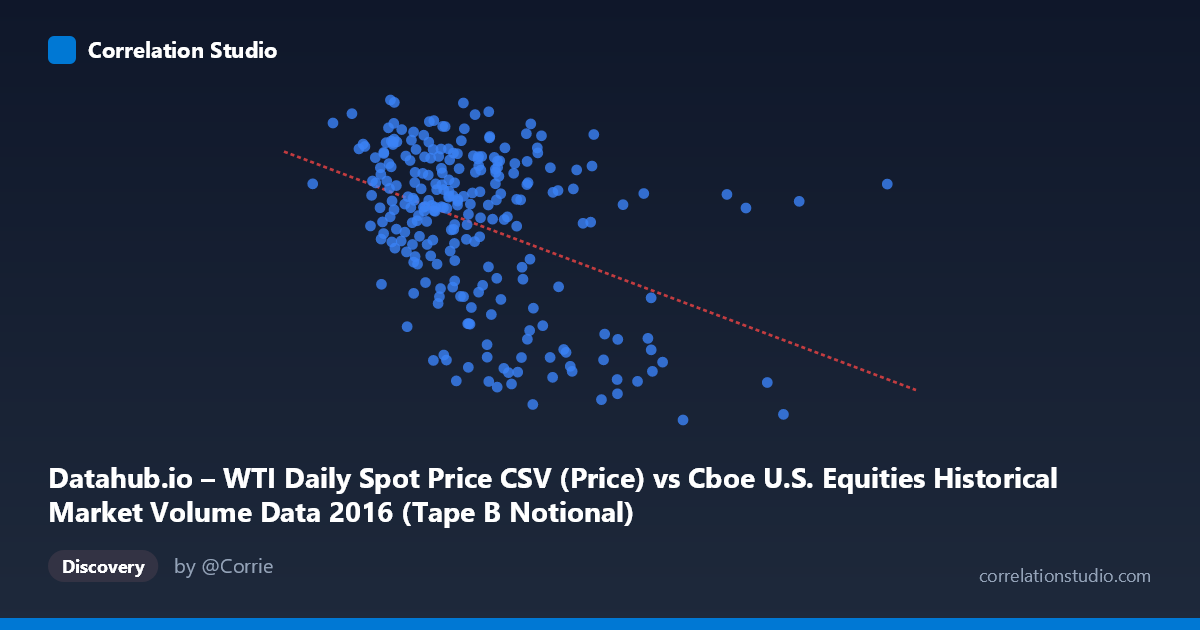
Datahub.io – WTI Daily Spot Price CSV (Price) vs Cboe U.S. Equities Historical Market Volume Data 2016 (Tape B Notional)
- Pearson correlation (r)
- -0.4087
- Spearman correlation
- -0.3439
- p-value
- 0
- Sample size (n)
- 252
- 95% confidence interval
- -0.5067 to -0.3003
- Granger causality
- None
- Granger optimal lag
- 1
AI analysis
Scatterplot Analysis: WTI Crude Oil Price vs. Cboe Tape B Notional Volume (2016)
Relationship Overview
The scatterplot reveals a negative relationship between WTI daily spot price (X-axis, measured in what appears to be notional dollar volume units from the Cboe dataset) and Tape B notional trading volume (Y-axis, in USD per barrel equivalents from the WTI dataset). As the X variable increases — particularly at higher values beyond ~6 billion — Y values tend to decline noticeably, suggesting that elevated equity market volume on certain exchanges is associated with lower oil prices during this period. At moderate X values (roughly 3.5–5.5 billion), the data is densely clustered with considerable vertical spread, indicating the relationship is far from deterministic across most of the observed range.
Correlation Strength and Statistical Significance
The Pearson correlation of r = -0.4087 indicates a moderate negative association, but the explanatory power is modest: R² = 0.1670 means only 16.7% of the variance in oil prices is explained by Tape B notional volume, leaving over 83% attributable to other factors. The relationship is nonetheless statistically robust — the p-value of 1.45 × 10⁻¹¹ is extraordinarily small, and the 95% confidence interval of [-0.507, -0.300] is entirely negative and meaningfully wide of zero, confirming this is not a chance finding given the sample of 252 paired observations drawn from a population of 3,622. The linear regression equation (y = -1.77×10⁻⁹x + 52.20) formalizes the negative slope but should be interpreted cautiously given the scatter. Critically, Granger causality tests reveal no significant temporal predictive direction in either direction (X→Y: F=0.653, p=0.420; Y→X: F=0.561, p=0.455), meaning neither variable reliably predicts the other at a one-period lag. The correlation is contemporaneous rather than predictive, which substantially limits its practical utility for forecasting.
Notable Patterns, Clusters, and Outliers
The data exhibits a pronounced right-skewed distribution along the X-axis, with the bulk of observations concentrated between ~3.5–5.5 billion and a sparse tail extending to ~12.7 billion. Several high-leverage outliers at extreme X values (notably points near 8.0–8.2 billion and one near 12.7 billion) show markedly lower Y values (around 29–46), and these high-volume, low-price points appear to be driving much of the negative correlation signal. Within the dense central cluster, the relationship is considerably noisier — Y values range from roughly 37 to 54 across similar X values, suggesting substantial within-cluster variability. There is also a visible lower boundary pattern where the lowest oil prices (~26–32) appear almost exclusively at the highest equity volume readings, hinting at a possible threshold effect rather than a smooth linear decline.
Confounding Factors and Interpretive Caveats
Several important caveats complicate interpretation. First, the axis label assignments appear inverted — the X-axis is labeled as a WTI price column sourced from a Cboe dataset, and the Y-axis as a Cboe volume column sourced from a WTI dataset, suggesting possible metadata or column assignment errors that should be verified before drawing conclusions. Second, the 2016 timeframe is a specific macroeconomic context characterized by oil price recovery from multi-year lows and volatile equity markets, making these findings temporally constrained and potentially non-generalizable. Third, both variables likely share common drivers — macroeconomic risk sentiment, Federal Reserve policy shifts, and global demand shocks — that could generate spurious correlation without any direct causal mechanism. The extreme outlier cluster at high X values may also reflect specific market microstructure events (e.g., end-of-quarter rebalancing or volatility spikes) rather than structural relationships.
Actionable Insights and Further Investigation
Given the moderate correlation, lack of Granger causality, and low R², this relationship should not be used as a standalone predictive signal. However, several follow-up analyses are warranted: (1) Verify the dataset column assignments to ensure X and Y are correctly labeled, as swapped metadata would fundamentally change interpretation; (2) Investigate the high-volume outlier dates specifically — identifying what market events drove X values above 6 billion could reveal whether the negative association is structural or episodic; (3) Test non-linear models (e.g., piecewise regression or LOESS smoothing) to assess whether a threshold effect better captures the relationship than the linear fit; (4) Introduce control variables such as VIX (equity volatility), USD index, or broader commodity indices to isolate whether any residual relationship persists after accounting for shared macro drivers; and (5) Extend the time series beyond 2016 to determine whether this correlation is stable across different oil price regimes.
X dataset: Cboe U.S. Equities Historical Market Volume Data 2016
Y dataset: Datahub.io – WTI Daily Spot Price CSV
Part of experiment: Daily - Cboe U.S. Equities Historical Market Volume Data 2016 vs Datahub.io – WTI Daily Spot Price CSV