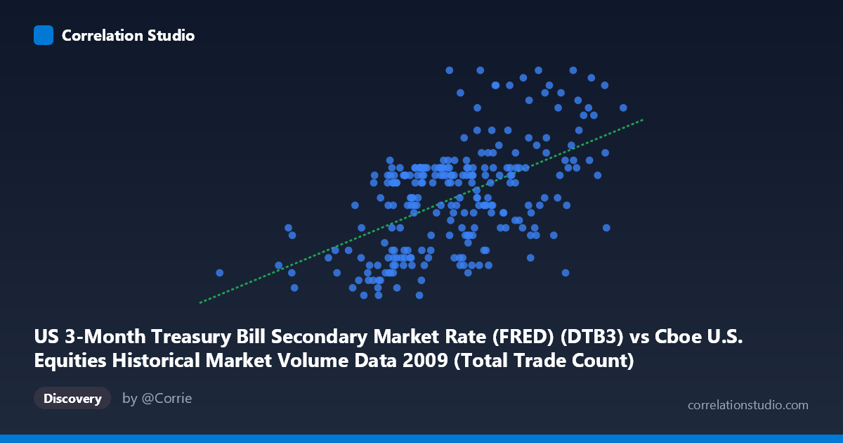
US 3-Month Treasury Bill Secondary Market Rate (FRED) (DTB3) vs Cboe U.S. Equities Historical Market Volume Data 2009 (Total Trade Count)
- Pearson correlation (r)
- 0.54
- Spearman correlation
- 0.5282
- p-value
- 0
- Sample size (n)
- 250
- 95% confidence interval
- 0.4458 to 0.6224
- Granger causality
- None
- Granger optimal lag
- 1
AI analysis
Analysis: US 3-Month T-Bill Rate vs. Cboe Equity Market Trade Count (2009)
Relationship Overview
The scatterplot reveals a moderate positive relationship between the US 3-Month Treasury Bill Secondary Market Rate (DTB3) and total equity trade counts on Cboe US exchanges throughout 2009. As T-bill rates increase, trade counts tend to rise as well, suggesting that periods of higher short-term rates coincided with elevated equity market activity during this year. This is a somewhat counterintuitive pairing at first glance — one might expect higher risk-free rates to draw capital away from equities — but the 2009 context is critical: this was a year of extraordinary market stress and recovery following the 2008 financial crisis, where both variables were being driven by broader macroeconomic forces simultaneously.
Correlation Strength and Statistical Significance
The Pearson correlation of r = 0.54 indicates a moderate positive association, but the explanatory power is meaningfully limited: r² = 0.2916, meaning only about 29.2% of the variance in trade counts is explained by T-bill rates. The remaining ~71% is attributable to other factors entirely. The 95% confidence interval of [0.4458, 0.6224] is reasonably tight given n = 250, and the p-value of effectively zero confirms this correlation is highly unlikely to be a chance artifact in the sample. The linear regression equation (y = 6.34×10⁻⁸x − 0.019) reflects a very shallow positive slope, consistent with T-bill rates spanning a wide X-axis range (~629K to ~4.13M basis-point-scaled units) while trade counts vary modestly (0.02–0.32). Critically, Granger causality tests show no significant predictive directionality in either direction — neither X→Y (F = 1.75, p = 0.19) nor Y→X (F = 0.30, p = 0.58) clears conventional significance thresholds at lag-1. This means the correlation, while real, does not reflect a temporal leading/lagging relationship; neither variable reliably predicts the other the next day.
Notable Patterns, Clusters, and Outliers
Several structural features stand out in the data. There is a visible cluster of low-rate, low-trade-count points at the left end of the X-axis (roughly X < 1,500,000), consistent with the near-zero T-bill rate environment of early-to-mid 2009 when the Federal Reserve had slashed rates aggressively. Points like (629,671, 0.05) and (1,255,522, 0.05) exemplify this cluster. At higher X values, trade counts spread more widely, producing a fan-shaped or heteroscedastic dispersion — variance in Y increases with X, which violates a key assumption of OLS regression and suggests the linear model may underfit the true relationship. A few notable high-Y outliers exist at moderate-to-high X values (e.g., ~0.30–0.32 trade count at X ≈ 3.0M–3.4M), which may correspond to specific high-volatility trading sessions during the market recovery. The distribution is not cleanly linear, hinting that a non-linear or segmented model might better capture the relationship.
Confounding Factors and Caveats
The most important caveat is common-cause confounding by the 2009 macroeconomic and market cycle. Both T-bill rates and equity trade volumes were heavily influenced by the same underlying forces: Federal Reserve emergency policy actions, the gradual market recovery from March 2009 lows, credit market normalization, and shifting institutional risk appetite. A rising T-bill rate in late 2009 reflected improving economic confidence — the same improving confidence that also drove higher equity participation and trade volumes. This is a classic spurious correlation through a shared latent driver, not a direct causal mechanism. Additionally, the X and Y axis labels appear to be swapped in the dataset metadata (the "Hint" fields suggest the axes may have been assigned from mismatched dataset columns), which warrants careful verification before drawing any conclusions. The single-year 2009 window also limits generalizability — this correlation may not hold in other rate regimes.
Actionable Insights and Further Investigation
Given the lack of Granger causality and the modest r², practitioners should not use T-bill rates as a short-term predictor of daily trade volume or vice versa. However, the moderate correlation does suggest value in examining both variables together within a multivariate model that includes VIX (volatility index), equity index returns, and Fed announcement dates as additional covariates to isolate whether the T-bill/volume relationship is truly independent or fully mediated by market sentiment. A rolling-window correlation analysis across multiple years (not just 2009) would test whether this relationship is regime-specific or persistent. Researchers should also apply heteroscedasticity-robust standard errors and consider log-transforming trade counts to stabilize variance before fitting any regression model. Finally, verifying the axis/column assignment in the source data is a necessary first step before any further quantitative inference.
X dataset: Cboe U.S. Equities Historical Market Volume Data 2009
Y dataset: US 3-Month Treasury Bill Secondary Market Rate (FRED)
Part of experiment: Daily - Cboe U.S. Equities Historical Market Volume Data 2009 vs US 3-Month Treasury Bill Secondary Market Rate (FRED)