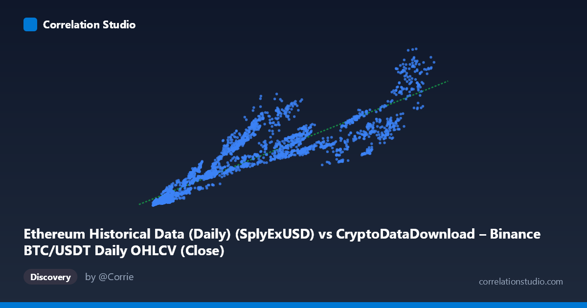
Ethereum Historical Data (Daily) (SplyExUSD) vs CryptoDataDownload – Binance BTC/USDT Daily OHLCV (Close)

Pearson correlation (r): 0.9056
Spearman correlation: 0.944
p-value: 0
Sample size (n): 3191
95% confidence interval: 0.8991 to 0.9116
Granger causality: None
Granger optimal lag: 10

AI analysis

Analysis of the X–Y Relationship

1. Overview of the Relationship

The scatterplot depicts a strong positive association between the X variable (labeled as Ethereum's SplyExUSD, though the values—ranging from ~3,189 to ~124,658—are inconsistent with actual ETH exchange-supply figures and more plausibly represent a price-like metric) and Y (labeled as BTC/USDT closing price, with values in the tens of billions, which is also inconsistent with actual BTC prices and suggests this may be a derived, aggregated, or mislabeled metric such as market cap or cumulative volume). Regardless of the labeling ambiguity, the data show a clear upward-sloping, roughly linear trend: as X increases, Y increases proportionally, with linear regression fitting y = 556,502x + 3.53 billion.

2. Strength, Direction, and Statistical Confidence

The correlation coefficient (r = 0.906) indicates a strong positive linear relationship, and r² = 0.820 means approximately 82% of the variance in Y is statistically explained by X — a substantial share, though nearly one-fifth of the variance remains unexplained by this single linear predictor. The 95% confidence interval [0.899, 0.912] is tight, and combined with p ≈ 0, this confirms the correlation is highly unlikely to be due to chance, given the large sample size (n = 3,191). However, correlation strength should not be conflated with causal direction: the Granger causality tests show no significant predictive relationship in either direction (X→Y: p = 0.877; Y→X: p = 0.825). This means that past values of X do not help forecast future Y, nor vice versa — the strong contemporaneous correlation likely stems from both variables responding to a shared external driver (e.g., overall crypto market cycles, macro liquidity conditions, or time-based trend) rather than one variable mechanically driving the other.

3. Patterns, Clusters, and Non-linear Features

The sample points suggest the relationship is not perfectly linear — at low X values (roughly 3,000–15,000), Y values cluster tightly and low (2–16 billion), showing a steep, almost proportional rise. In the mid-to-upper range (X 60,000), Y values show wider dispersion at similar X levels (e.g., X≈62,000–66,000 yields Y between 31–42 billion; X≈83,000–90,000 yields Y between 27–55 billion), indicating heteroskedasticity — variance in Y grows with X. This fanning-out pattern implies the linear model fits the lower range better than the upper range, and a log-log or power-law model might capture the relationship more accurately, especially if both series reflect exponential/multiplicative growth dynamics typical of crypto asset valuations.

4. Confounding Factors and Caveats

Since both variables are cryptocurrency-related metrics from overlapping time periods (2017–2026), they are both likely driven by shared macro factors: overall market sentiment, BTC dominance cycles, regulatory news, and liquidity conditions across the entire crypto ecosystem. This makes spurious correlation via a common trend or time confound highly plausible — bull/bear market cycles could inflate both series simultaneously without direct causal linkage. Additionally, the mismatched value ranges and labels (SplyExUSD reaching only 5-digit values, "Close" price in the billions) suggest possible data misalignment, unit conversion issues, or that these columns represent aggregated/derived metrics (e.g., total supply value or market cap) rather than raw prices — this should be verified before drawing economic conclusions.

5. Recommendations for Further Investigation

To clarify the relationship: (1) verify column definitions and units to rule out mislabeling or scaling errors; (2) test a log-transformed or power-law regression model to address the observed heteroskedasticity and improve fit in the upper range; (3) since Granger tests show no lead-lag predictability, consider testing for cointegration (e.g., Engle-Granger or Johansen tests) to check for a long-run equilibrium relationship despite the lack of short-term causality; and (4) introduce a third shared control variable (e.g., total crypto market cap or a liquidity index) to test whether the observed correlation is spurious or mediated by common macro-crypto trends.

X dataset: CryptoDataDownload – Binance BTC/USDT Daily OHLCV

Y dataset: Ethereum Historical Data (Daily)

Part of experiment: Bitcoin - CryptoDataDownload – Binance BTC/USDT Daily OHLCV vs Ethereum Historical Data (Daily)