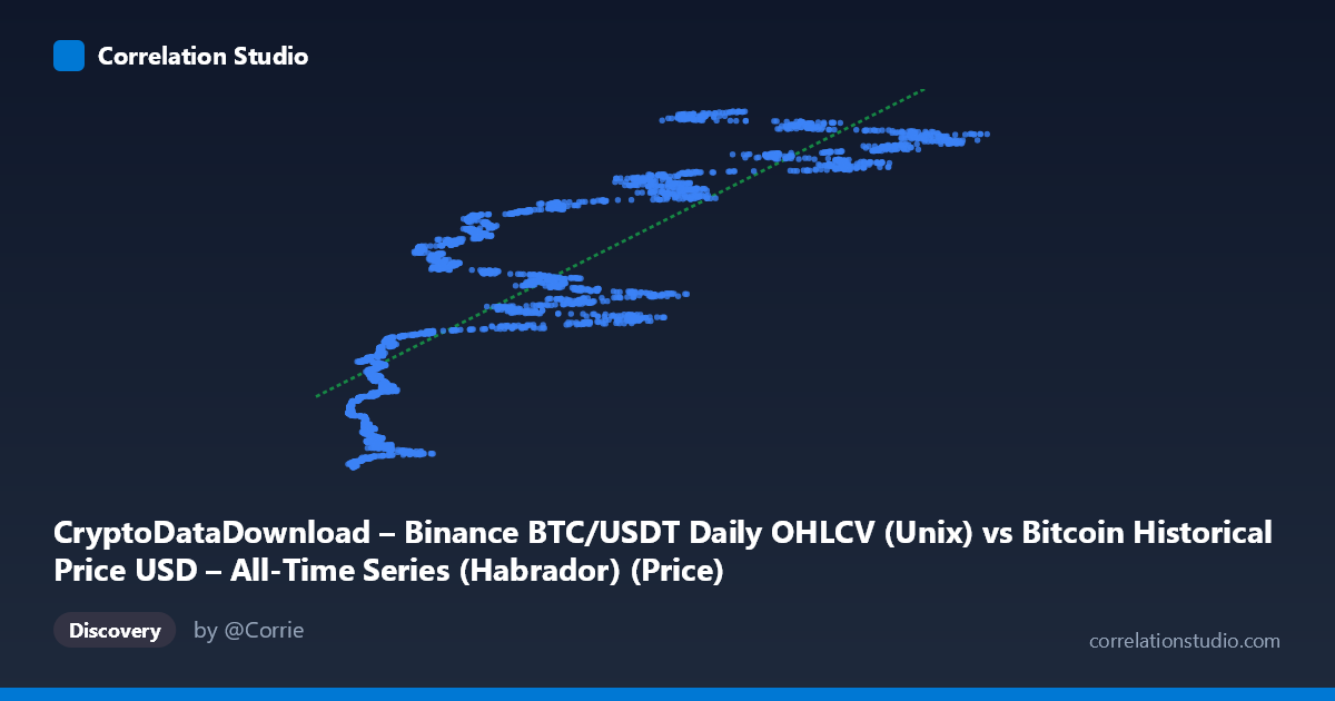
CryptoDataDownload – Binance BTC/USDT Daily OHLCV (Unix) vs Bitcoin Historical Price USD – All-Time Series (Habrador) (Price)
- Pearson correlation (r)
- 0.8407
- Spearman correlation
- 0.8864
- p-value
- 0
- Sample size (n)
- 3169
- 95% confidence interval
- 0.8301 to 0.8506
- Granger causality
- None
- Granger optimal lag
- 10
- Time coverage
- 2017-08-17 to 2026-04-28
AI analysis
Analysis: BTC Price vs. Unix Timestamp Correlation
1. What the Visualization Reveals
This scatterplot is somewhat unusual in that the X-axis is not truly an independent variable in the conventional sense — it's a Bitcoin price column ("CryptoDataDownload OHLCV") being plotted against a Unix timestamp column relabeled as "Price" from a separate Habrador dataset. Effectively, this chart is showing how BTC's historical price level relates to the calendar date on which it occurred (encoded numerically as epoch time). The visualization is essentially a price-vs-time chart in disguise, which explains why the pattern resembles Bitcoin's well-known multi-cycle growth trajectory rather than a relationship between two independent economic variables.
2. Strength, Direction, and Statistical Confidence
The correlation (r = 0.84, r² = 0.71) is strong and positive, meaning that 71% of the variance in the Y-values (timestamps) can be linearly explained by X (price). The tight confidence interval [0.830, 0.851] and p-value of essentially 0 indicate this relationship is highly statistically robust and not a product of sampling noise — with n=3,169 points, even modest correlations would reach significance, but here the effect size itself is large. However, r² of 0.71 also means 29% of variance is unexplained by a simple linear fit, which is substantial given the data's known non-linear (exponential/logarithmic) growth pattern.
Critically, the Granger causality tests show no significant predictive direction in either direction (X→Y: p=0.35; Y→X: p=0.11), even at an optimal lag of 10 periods. This is expected and important: since X and Y are essentially the same underlying phenomenon (BTC price) viewed through two different data pipelines/timestamps, there is no meaningful "causal" lead-lag relationship to detect — correlation here reflects structural/definitional overlap, not one variable driving another.
3. Notable Patterns and Non-Linear Features
The sample points reveal Bitcoin's classic stair-step, multi-cycle growth pattern: long stretches of relatively flat/low prices (2017–2020, in the $4,000–$12,000 range) followed by steep parabolic run-ups (2021, 2024–2025) reaching $100,000+. This is inherently non-linear (closer to exponential or log-linear), so a straight-line fit (y = 2.05E6·x + 1.56E12) will systematically underfit the flat bear-market periods and overfit/underfit the sharp bull-market spikes. Visually, expect clustering at both low-X/early-timestamp and high-X/late-timestamp extremes, with sparser, more scattered data in the volatile mid-range ($40K–$70K) where BTC has traded during multiple different cycles (2021 crash, 2024 consolidation) — meaning the same price level maps to multiple different time periods, injecting vertical scatter/noise into the trend.
4. Confounding Factors and Caveats
The most important caveat: this is likely a data-merging artifact rather than a genuine bivariate relationship. Both columns trace back to Bitcoin price history from different sources (Habrador dataset and Binance CDD), joined seemingly by row-index rather than by matching dates — meaning "X" and "Y" may not correspond to the same day's price, creating spurious alignment issues. Additionally, price-vs-time relationships in financial assets violate standard regression assumptions (autocorrelation, non-stationarity, heteroscedasticity — variance clearly increases at higher price levels), making the r²/p-value interpretation less meaningful in a causal sense than it would be for independent economic variables.
5. Suggested Next Steps
1. Verify the data join: Confirm whether X and Y rows are matched by actual trade date rather than arbitrary row order — mismatched timestamps would explain scatter and weaken true correlation. 2. Re-run with proper date alignment and use actual date/price columns (not two separate "price-like" fields) to test genuine cross-exchange price parity (e.g., Binance vs. another source) rather than price-vs-time. 3. Apply log transformation to price before fitting, given BTC's exponential growth character — this would likely raise r² substantially and better reflect the true trend. 4. Segment by market cycle (2017-18, 2020-21, 2022 bear, 2023-25 bull) to check whether the relationship is stable or regime-dependent, since pooling all cycles into one linear fit obscures cycle-specific dynamics.
X dataset: Bitcoin Historical Price USD – All-Time Series (Habrador)
Y dataset: CryptoDataDownload – Binance BTC/USDT Daily OHLCV
Part of experiment: Bitcoin - Bitcoin Historical Price USD – All-Time Series (Habrador) vs CryptoDataDownload – Binance BTC/USDT Daily OHLCV