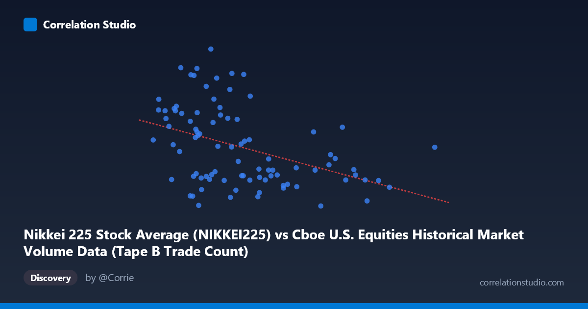
Nikkei 225 Stock Average (NIKKEI225) vs Cboe U.S. Equities Historical Market Volume Data (Tape B Trade Count)
- Pearson correlation (r)
- -0.4188
- Spearman correlation
- -0.4388
- p-value
- 0.00004
- Sample size (n)
- 90
- 95% confidence interval
- -0.5759 to -0.2318
- Granger causality
- None
- Granger optimal lag
- 10
AI analysis
Analysis: Nikkei 225 vs. Cboe Tape B Trade Count
Relationship Overview
The scatterplot reveals a modest negative relationship between the Nikkei 225 stock index level and Cboe U.S. Equities Tape B Trade Count over the January–May 2026 period. The linear regression equation (y = -0.00578506x + 62,169) indicates that as the Nikkei 225 rises, Tape B trade counts tend to decline slightly. Visually, the data points are broadly dispersed across the plot with a gentle downward slope, suggesting the relationship exists but is far from deterministic. The wide spread of Y values (ranging from ~51,000 to ~65,000 trades) at any given X value reinforces that Nikkei 225 levels alone offer limited predictive power for U.S. Tape B activity.
Correlation Strength and Statistical Significance
The correlation coefficient of r = -0.4188 indicates a weak-to-moderate negative association. Critically, R² = 0.1754 means that only 17.5% of the variance in Tape B Trade Count is explained by the Nikkei 225 level — leaving over 82% attributable to other factors entirely. The 95% confidence interval for r spans [-0.5759, -0.2318], which is meaningfully wide, reflecting genuine uncertainty about the true population correlation magnitude, though the interval does not cross zero. The p-value of 3.99×10⁻⁵ confirms the correlation is statistically significant at conventional thresholds given the population size of N = 1,980. However, Granger causality testing finds no significant predictive direction in either direction — neither X→Y (F = 1.88, p = 0.066) nor Y→X (F = 1.01, p = 0.449) achieves significance at the 5% level. This is a critical qualifier: the Nikkei 225 does not temporally predict Tape B trade counts, and vice versa, meaning the observed correlation likely reflects coincidental co-movement rather than any causal or leading-indicator relationship.
Notable Patterns and Outliers
Several features stand out in the data. There is a visible cluster of points in the X range of approximately 800,000–1,100,000 with highly dispersed Y values (from ~51,000 to ~65,000), suggesting high variability in Tape B activity during mid-range Nikkei levels. At higher Nikkei values (above ~1,400,000), the Y values appear more compressed in the lower range (~51,000–58,000), which drives the negative slope. A few potential outliers merit attention: the point near (892,624, 64,996) represents an unusually high Tape B count for its Nikkei level, and the point at (1,808,757, 56,279) sits far to the right on the X-axis as an extreme Nikkei observation. The lower-left region (low Nikkei, lower trade counts) also shows some atypical values like (1,342,474, 51,064) — a relatively high Nikkei paired with a very low trade count.
Confounding Factors and Caveats
Several important caveats apply to this analysis. First, the datasets appear to be mismatched by description — the X-axis label references Nikkei 225 values drawn from a Cboe volume dataset, and the Y-axis references Tape B Trade Count drawn from a Nikkei dataset, raising concerns about data provenance and potential labeling artifacts. Second, the negative correlation could easily be spurious, driven by shared time trends: if U.S. equity trading volumes were trending downward over this period while Nikkei 225 levels were rising, a mechanical negative correlation would emerge without any genuine economic linkage. Third, day-of-week effects, U.S. and Japanese market holidays, and macroeconomic announcements affecting both markets simultaneously could all generate correlated fluctuations. The optimal Granger lag of 10 periods also warrants scrutiny — this is a relatively long lag that may reflect over-fitting rather than a genuine economic transmission mechanism.
Actionable Insights and Further Investigation
Given the weak explanatory power and absent Granger causality, practitioners should avoid using Nikkei 225 levels as a predictive signal for Tape B Trade Count in isolation. Several follow-up analyses are warranted: (1) Detrend both series to test whether the correlation survives removal of common time trends, which would sharply clarify whether the relationship is genuine or spurious; (2) Incorporate additional covariates such as VIX levels, overall U.S. market volume, or USD/JPY exchange rates to assess whether the Nikkei-Tape B relationship is a proxy for broader risk-on/risk-off sentiment; (3) Test shorter lag windows in Granger causality (1–5 periods) to check whether intraday or next-day spillover effects exist that the 10-period optimal lag might be masking; and (4) Verify data alignment and labeling to ensure the X and Y series are correctly matched to their respective sources before drawing any operational conclusions.
X dataset: Cboe U.S. Equities Historical Market Volume Data
Y dataset: Nikkei 225 Stock Average
Part of experiment: Daily - Cboe U.S. Equities Historical Market Volume Data vs Nikkei 225 Stock Average