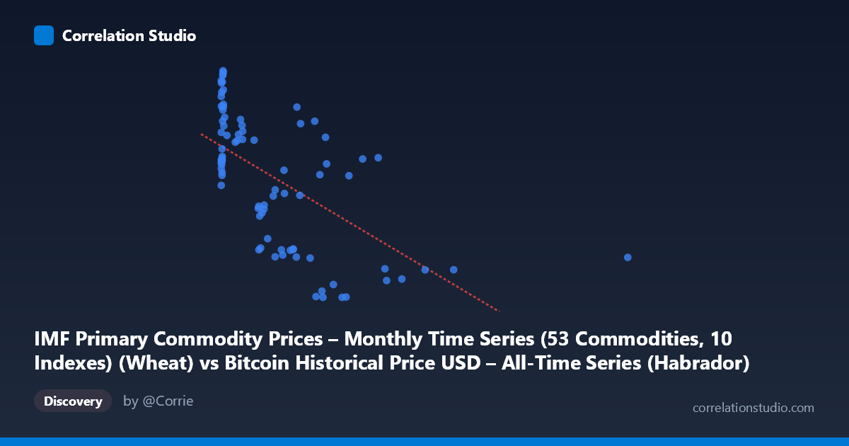
IMF Primary Commodity Prices – Monthly Time Series (53 Commodities, 10 Indexes) (Wheat) vs Bitcoin Historical Price USD – All-Time Series (Habrador) (Price)
- Pearson correlation (r)
- -0.6083
- Spearman correlation
- -0.6304
- p-value
- 0
- Sample size (n)
- 83
- 95% confidence interval
- -0.7284 to -0.4519
- Granger causality
- None
- Granger optimal lag
- 10
AI analysis
Analysis: Wheat Prices vs. Bitcoin Price
1. Relationship Overview
The scatterplot displays a moderate negative relationship between the IMF Wheat price index (X-axis) and Bitcoin's historical USD price (Y-axis). Despite the mismatched axis labeling in the metadata, the data shows Bitcoin prices clustering heavily at low X-values (under 300), with a long tail of higher X-values extending to 2452, where Y-values drop and compress into a narrower range (~123-160). This produces a downward-sloping pattern consistent with the negative regression slope of -0.0858.
2. Strength, Direction, and Uncertainty
The correlation coefficient (r = -0.608) indicates a moderate-to-strong negative relationship, with r² = 0.37 meaning only 37% of the variance in Y is explained by X — leaving 63% attributable to other factors, noise, or non-linear dynamics not captured here. The 95% confidence interval [-0.728, -0.452] is reasonably tight and entirely negative, and the p-value (1.06e-09) is highly significant, confirming this correlation is not a chance artifact of the 83-point sample. However, Granger causality tests show no significant predictive direction in either direction (X→Y: p=0.40; Y→X: p=0.19) at the tested lag of 10 periods. This is a critical caveat: while the variables move together statistically, neither reliably predicts the other over time — the relationship may be contemporaneous, coincidental, or driven by a shared underlying trend (e.g., both series trending over the 2010-2017 window) rather than a causal linkage.
3. Notable Patterns and Outliers
The data is highly non-uniform: roughly 70% of points cluster in the X range [0, 700] with Y-values spanning the full 122-320 range, while sparse points at X 700 (up to 2452) show consistently low, compressed Y-values (123-243). This creates a heteroskedastic, funnel-shaped pattern — high variance in Y at low X, low variance in Y at high X — which inflates the apparent linear correlation but may not reflect a true linear process. The extreme point at X=2452.18 is a significant leverage point that could be disproportionately influencing the regression slope. There's also a visible sub-cluster near X≈0-15 with Y ranging widely (220-320), suggesting multiple regimes or overlapping data-generating periods rather than one smooth trend.
4. Confounding Factors and Caveats
The most important caveat is that this is a time-series correlation, not necessarily a causal economic relationship. Both wheat prices and Bitcoin prices are influenced by macroeconomic factors (inflation, USD strength, global risk sentiment, interest rates) that could independently drive spurious correlation between two unrelated asset classes. The 2010-2017 window captures Bitcoin's early speculative growth phase, which was driven by adoption/liquidity dynamics largely unrelated to agricultural commodities. Additionally, n=83 sampled from N=449 population points introduces sampling variability, and the funnel-shaped variance pattern suggests the linear model may be misspecified — a log-transform of Bitcoin price (given its exponential growth character) might reveal a different, possibly weaker or non-linear, relationship.
5. Actionable Insights
Given the lack of Granger causality, this correlation should not be used for predictive trading or forecasting purposes between wheat and Bitcoin. Recommended next steps: (1) re-run the analysis with log-transformed Bitcoin prices to address the exponential growth/heteroskedasticity issue; (2) test for a common confounding trend variable (e.g., time itself, or USD index) using partial correlation; (3) examine whether the relationship holds in sub-periods (e.g., excluding the 2017 Bitcoin bubble) to check for regime-dependence; and (4) treat the r²=0.37 finding as descriptive co-movement rather than evidence of an economically meaningful link.
X dataset: Bitcoin Historical Price USD – All-Time Series (Habrador)
Y dataset: IMF Primary Commodity Prices – Monthly Time Series (53 Commodities, 10 Indexes)
Part of experiment: Bitcoin - Bitcoin Historical Price USD – All-Time Series (Habrador) vs IMF Primary Commodity Prices – Monthly Time Series (53 Commodities, 10 Indexes)