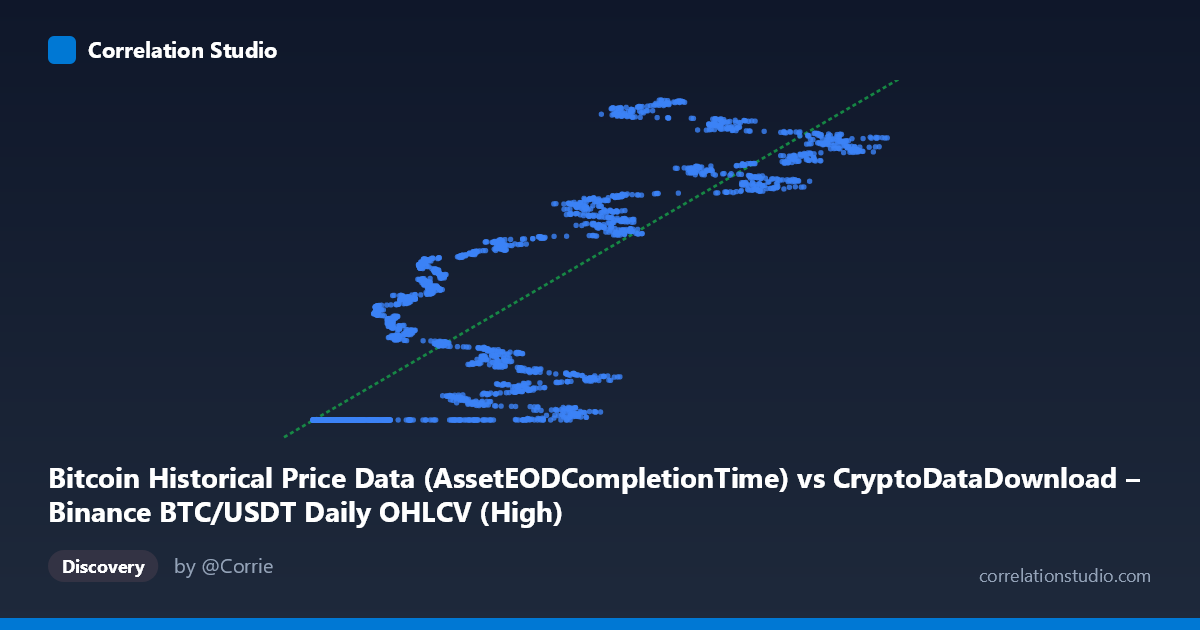
Bitcoin Historical Price Data (AssetEODCompletionTime) vs CryptoDataDownload – Binance BTC/USDT Daily OHLCV (High)
- Pearson correlation (r)
- 0.85
- Spearman correlation
- 0.886
- p-value
- 0
- Sample size (n)
- 3191
- 95% confidence interval
- 0.8401 to 0.8593
- Granger causality
- None
- Granger optimal lag
- 10
AI analysis
Analysis of Bitcoin Price Data Correlation
1. What the Visualization Reveals
This scatterplot compares two variables that both derive from the same underlying asset (Bitcoin/USDT price on Binance), which explains the strong positive relationship. The X-axis appears to capture a timestamp-like or index-derived value (labeled as "AssetEODCompletionTime" but ranging numerically like an index or derived metric from 3,276 to 126,200), while Y represents the daily high price. The data shows a clear upward trend, but importantly, the pattern is not a simple straight line — there's evident clustering and step-like behavior, particularly a dense horizontal band around Y ≈ 1,614,337,000–1,614,338,000 that appears repeatedly across many different X values (especially at low X). This suggests a data artifact: many records share nearly identical Y values (likely a placeholder, minimum bound, or repeated timestamp) despite varying X, which is not representative of true price dynamics.
2. Strength, Direction, and Statistical Confidence
The correlation coefficient (r = 0.85, r² = 0.72) indicates a strong positive linear relationship, with 72.25% of the variance in Y statistically explained by X. The tight confidence interval [0.840, 0.859] and p-value of ~0 confirm this correlation is highly reliable and not due to chance, given the large sample size (n=3,191). However, the remaining 28% of variance is unexplained, meaning X alone is an incomplete predictor of Y — other factors or nonlinear dynamics are at play.
Critically, the Granger causality test shows no significant predictive direction in either direction (X→Y: p=0.31; Y→X: p=0.13). This means that despite the strong contemporaneous correlation, neither variable temporally leads the other in a statistically meaningful way at the tested lag (10 periods). This is a crucial distinction: strong correlation ≠ causation or predictability. The relationship is likely driven by both variables reflecting the same underlying price trend simultaneously, rather than one causing changes in the other over time.
3. Notable Patterns and Anomalies
The most striking feature is the plateau/clustering effect at Y ≈ 1.614B occurring across a wide range of X values (roughly 3,800–25,000), suggesting these points correspond to the early history of the dataset (2017-08-17 start date) where price data may be flat, backfilled, or minimally varying day-to-day. Beyond this cluster, the relationship becomes more dispersed and appears piecewise or non-linear — segments show different slopes (e.g., rapid rise from X≈60,000 to X≈90,000, plateauing again near X≈100,000+). This suggests the relationship may be better modeled by a piecewise or logarithmic function rather than pure linear regression, especially given that Bitcoin prices exhibit exponential growth phases and consolidation periods.
4. Confounding Factors and Caveats
Several caveats warrant attention: - Same-asset autocorrelation: Both variables derive from Bitcoin/BTC-USDT price data, so high correlation is somewhat mechanically expected rather than revealing a novel economic relationship. - Time-series non-stationarity: Bitcoin prices are highly non-stationary (trending, volatile, regime-switching). Standard Pearson correlation and linear regression assume stationarity and linearity, which are violated here — inflating apparent "explanatory power" while masking structural breaks. - The early flat-cluster (2017 data) may distort the regression line, pulling it to fit an artifact rather than genuine variation. - Different data sources/licensing for X and Y (despite similar descriptions) raises questions about whether these are truly independent measurements or redundant/derived fields — this could artificially inflate r².
5. Suggestions for Further Investigation
- Decompose by time regime: Split data into bull/bear/consolidation periods and re-run correlation/regression to check for parameter stability. - Test for cointegration rather than relying on Pearson r/Granger causality alone, given both series are likely non-stationary price series — cointegration testing (e.g., Engle-Granger) is more appropriate for this data type. - Investigate the flat cluster: Determine why ~15-20% of points show nearly identical Y despite varying X — likely a data quality/backfill issue that should be cleaned or excluded before re-analysis. - Log-transform both axes to test whether the relationship is better characterized as log-linear (common in asset price analysis) versus the current linear fit. - Clarify variable definitions: Confirm what X actually represents (timestamp vs. derived index) before drawing further economic conclusions, since the axis label is ambiguous relative to the numeric range shown.
X dataset: CryptoDataDownload – Binance BTC/USDT Daily OHLCV
Y dataset: Bitcoin Historical Price Data
Part of experiment: Bitcoin - CryptoDataDownload – Binance BTC/USDT Daily OHLCV vs Bitcoin Historical Price Data