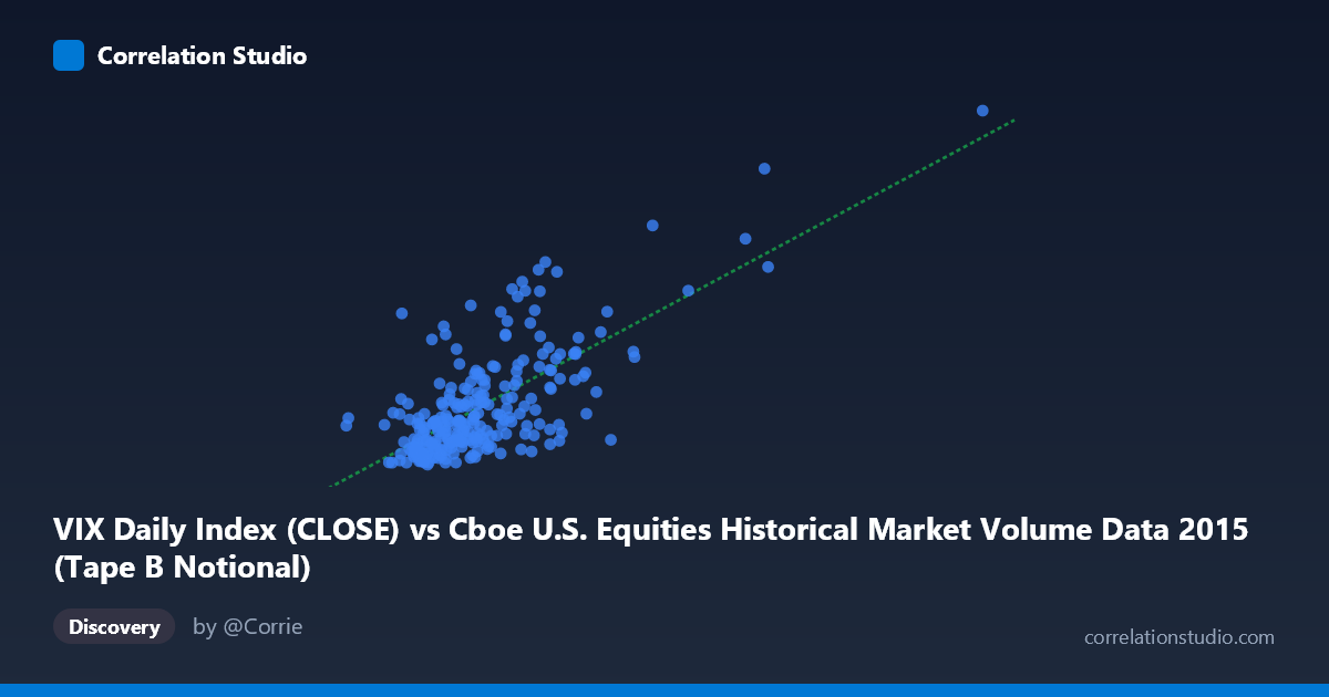
VIX Daily Index (CLOSE) vs Cboe U.S. Equities Historical Market Volume Data 2015 (Tape B Notional)

Pearson correlation (r): 0.7071
Spearman correlation: 0.5903
p-value: 0
Sample size (n): 252
95% confidence interval: 0.6394 to 0.7639
Granger causality: None
Granger optimal lag: 1
Time coverage: 2015-01-02 to 2015-12-31
Recomputed on refreshed data: 2026-10-09 (r was 0.7071)

AI analysis

Scatterplot Analysis: VIX Daily Index vs. Tape B Notional Volume (2015)

Relationship Overview

The scatterplot reveals a moderately strong positive relationship between the CBOE Volatility Index (VIX) closing values and Tape B Notional trading volume across U.S. equity exchanges in 2015. As VIX levels rise — indicating greater market fear or uncertainty — Tape B Notional volume tends to increase correspondingly. This is a financially intuitive finding: elevated volatility typically drives higher trading activity as market participants reposition, hedge, or react to uncertainty. The linear regression equation (y = 1.76 × 10⁻⁹x + 7.06) confirms a positive slope, though the extremely small coefficient reflects the vast scale difference between the two variables (VIX in single/double digits vs. notional values in billions).

Correlation Strength and Statistical Significance

With r = 0.707 and r² = 0.50, exactly half of the variance in Tape B Notional volume is explained by VIX levels — a meaningfully substantial relationship by social science standards, though it equally underscores that the other 50% of variance is driven by factors outside this model. The 95% confidence interval of [0.639, 0.764] is relatively tight and does not approach zero, providing strong statistical confidence in the direction and approximate magnitude of this association. The p-value of effectively 0 across a paired sample of 252 observations drawn from a population of 3,302 trading records leaves no doubt about statistical significance. However, Granger causality analysis complicates the narrative considerably: neither direction (X→Y: F = 0.017, p = 0.896; Y→X: F = 0.025, p = 0.875) achieves significance, meaning that despite a robust contemporaneous correlation, neither variable demonstrably predicts the other with a one-period lag. This dissociation between correlation and temporal predictability is a critical caveat — the two variables move together, but neither reliably leads the other.

Notable Patterns, Clusters, and Outliers

The sample points reveal several important structural features. The bulk of observations cluster in a lower-left zone where VIX values fall roughly between 3.0–6.5 billion (notional) and VIX readings of 12–20, suggesting these represent typical 2015 market conditions. A second, sparser cluster emerges at higher VIX levels (25–30+) with correspondingly elevated notional volumes, consistent with the volatility spikes of August 2015 (the "Flash Crash" period). Several pronounced outliers are visible at extreme X values — notably points near 12.5–17.9 billion notional — that carry outsized influence on the regression slope. The point at approximately (12,491,974,396; 36.02) is particularly notable, representing an extreme joint observation that likely corresponds to a specific high-stress market event. The scatter also appears to fan outward at higher VIX values (heteroscedasticity), suggesting the relationship is less precise during high-volatility regimes.

Confounding Factors and Interpretive Caveats

Several important caveats apply. First, axis labeling appears inverted relative to conventional analysis: VIX (a volatility index) is placed on the X-axis while notional volume (from the market volume dataset) is labeled as the Y-axis, yet the dataset descriptions suggest the column assignments may be transposed — this warrants verification before drawing directional conclusions. Second, 2015 was not a typical year; it contained the August 2015 equity selloff, which likely inflates both variables simultaneously and could be driving much of the observed correlation through a handful of extreme events rather than a stable structural relationship. Third, Tape B specifically covers NYSE American and regional exchanges, so generalizing to total market behavior should be done cautiously. Finally, the absence of Granger causality at lag-1 may reflect that the relevant lag structure is intraday or multi-day, not captured by daily periodicity.

Actionable Insights and Further Investigation

Practitioners and researchers should consider several next steps. Testing multiple lag structures (2–5 periods) in the Granger causality framework could reveal delayed predictive relationships not captured at lag-1. Segmenting the analysis by excluding the August 2015 volatility episode would clarify whether the correlation holds in calmer regimes or is predominantly event-driven. Given the apparent heteroscedasticity, a log-log transformation of both variables could stabilize variance and potentially reveal a more consistent power-law relationship. Expanding the analysis to Tape A and Tape C notional volumes would test whether the VIX-volume relationship is Tape B-specific or market-wide. Finally, incorporating additional covariates — such as bid-ask spreads, options open interest, or macroeconomic releases — into a multivariate model could account for a meaningful portion of the unexplained 50% variance and move analysis closer to causal inference.

X dataset: Cboe U.S. Equities Historical Market Volume Data 2015

Y dataset: VIX Daily Index

Part of experiment: Daily - Cboe U.S. Equities Historical Market Volume Data 2015 vs VIX Daily Index