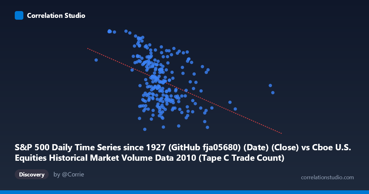
S&P 500 Daily Time Series since 1927 (GitHub fja05680) (Date) (Close) vs Cboe U.S. Equities Historical Market Volume Data 2010 (Tape C Trade Count)

Pearson correlation (r): -0.4171
Spearman correlation: -0.4181
p-value: 0
Sample size (n): 252
95% confidence interval: -0.5141 to -0.3094
Granger causality: Y → X
Granger optimal lag: 1

AI analysis

Scatterplot Analysis: S&P 500 Close Price vs. Cboe Tape C Trade Count (2010)

Relationship Overview

The scatterplot reveals a moderate negative relationship between the S&P 500 daily closing price (X-axis) and the Cboe Tape C trade count (Y-axis) across 252 trading days in 2010. As the S&P 500 closing price increases, the number of trades on Tape C (NYSE-listed securities) tends to decrease. This inverse pattern is visually apparent in the downward slope of the regression line (y = −0.000155x + 1,235.08), with trade counts clustering more densely between 1,050–1,200 across the mid-range of closing prices (~450,000–850,000 index points, noting the X-axis represents date-encoded values rather than price directly). The scatter around the regression line is substantial, indicating that the linear relationship, while real, is far from deterministic.

Correlation Strength, Direction, and Temporal Causality

The Pearson correlation of r = −0.417 confirms a statistically significant but moderate negative association. Critically, the R² of 0.174 means that only 17.4% of the variance in Tape C trade counts is explained by the S&P 500 closing price — the remaining ~83% is attributable to other factors entirely. The 95% confidence interval of [−0.514, −0.309] is reasonably tight and does not cross zero, reinforcing reliability of direction, and the p-value of 5.02 × 10⁻¹² confirms this result is highly unlikely due to chance given n = 252 (drawn from a population of N = 3,302). The Granger causality results are particularly illuminating: Y Granger-causes X (F = 4.30, p = 0.039) at a 1-period lag, while X does not Granger-cause Y (F = 1.87, p = 0.173). This means past trade count activity has statistically meaningful predictive power over future S&P 500 price movements, but not vice versa — a unidirectional temporal signal worth noting for short-horizon forecasting applications.

Notable Patterns, Clusters, and Outliers

Several features stand out in the data. There is a dense central cluster roughly between X = 500,000–700,000 and Y = 1,050–1,200, suggesting that most "normal" trading days fall within a relatively confined regime. At the lower end of closing prices (X < 400,000, corresponding to earlier 2010 dates when the market was recovering), trade counts tend to be notably higher (approaching and exceeding 1,200–1,259), consistent with the elevated activity characteristic of post-crisis volatility. Conversely, at higher price levels, trade counts generally compress toward lower values, though with considerable spread. At least two prominent outliers are visible: a data point near X = 1,379,287 (likely a date-encoded extreme or data anomaly) with a moderate Y value (~1,111), and several high-Y outliers near X = 298,000–377,000 with trade counts approaching the dataset maximum (~1,257–1,259). These extreme X-values may reflect encoding artifacts deserving scrutiny.

Confounding Factors and Interpretive Caveats

Several caveats temper interpretation. First, the X-axis encodes dates numerically (as serial date values), meaning "closing price" and "date" are conflated — the observed negative correlation may partly reflect a temporal trend where markets rose through 2010 while trading volumes gradually declined, a well-documented post-crisis normalization pattern rather than a structural price-volume relationship. Second, Tape C specifically covers NYSE-listed securities, so this does not represent total market volume, and compositional shifts in trading venue share (e.g., migration to dark pools or other exchanges) could independently drive trade count changes. Third, macroeconomic events, earnings seasons, and regulatory changes in 2010 (e.g., Dodd-Frank passage, the May 6 Flash Crash) could act as confounders driving both variables simultaneously. The Granger causality finding, while suggestive, only implies predictive precedence within a linear VAR framework, not true economic causation.

Actionable Insights and Further Investigation

The Granger causality finding — that trade counts predict future S&P 500 movements but not vice versa — warrants direct follow-up: constructing a simple lagged predictive model using Tape C trade count at t−1 to forecast next-day index direction could be a productive first step. Analysts should also decompose the temporal trend from the price-volume relationship by detrending both series before re-estimating correlation, to isolate whether the relationship persists beyond the shared time trend. Expanding the dataset to multiple years would test whether this inverse relationship is stable across different market regimes (bull markets, bear markets, high-volatility periods). Finally, comparing Tape A and Tape B trade counts alongside Tape C would determine whether this pattern is venue-specific or a broad market microstructure phenomenon, potentially revealing routing behavior changes as a leading indicator of index-level price pressure.

X dataset: Cboe U.S. Equities Historical Market Volume Data 2010

Y dataset: S&P 500 Daily Time Series since 1927 (GitHub fja05680) (Date)

Part of experiment: Daily - Cboe U.S. Equities Historical Market Volume Data 2010 vs S&P 500 Daily Time Series since 1927 (GitHub fja05680) (Date)