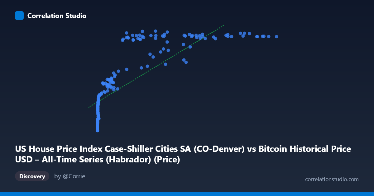
US House Price Index Case-Shiller Cities SA (CO-Denver) vs Bitcoin Historical Price USD – All-Time Series (Habrador) (Price)
- Pearson correlation (r)
- 0.7931
- Spearman correlation
- 0.9525
- p-value
- 0
- Sample size (n)
- 191
- 95% confidence interval
- 0.7337 to 0.8404
- Granger causality
- None
- Granger optimal lag
- 9
- Time coverage
- 2010-08-01 to 2026-06-01
- Recomputed on refreshed data
- 2026-10-24 (r was 0.7892)
AI analysis
Analysis: Bitcoin Price vs. Denver Case-Shiller Home Price Index
1. What the Visualization Reveals
The scatterplot shows a strong positive association between Bitcoin's historical USD price and the Denver Case-Shiller Home Price Index, but the relationship is clearly non-linear. At low Bitcoin prices (under ~$1,000), the Case-Shiller index clusters tightly between 123–200, showing very little sensitivity to small changes in Bitcoin's price. As Bitcoin climbs into the tens of thousands, the home price index rises and then flattens/saturates in the 300–325 range, even as Bitcoin continues to swing wildly up to $118,670. This produces a curve resembling a logarithmic or power-law shape rather than a straight line — consistent with the note that Spearman's ρ exceeds Pearson's r.
2. Strength, Direction, and Uncertainty
The Pearson correlation (r = 0.785, R² = 0.616) indicates a strong positive linear relationship, with about 62% of the variance in the housing index statistically explained by Bitcoin price. The 95% CI [0.723, 0.834] is fairly tight and excludes zero, and the p-value is effectively 0, so the correlation is highly unlikely to be a statistical fluke given this sample. However, statistical significance does not imply mechanism: the Granger causality tests show no significant predictive direction in either direction (X→Y: p=0.585; Y→X: p=0.785) at the optimal lag of 9 periods. This strongly suggests the correlation is not causal in a temporal, predictive sense — neither variable "leads" the other in a way that improves forecasting. Instead, both series likely trend upward together over the 2010–2026 window due to shared macro drivers (time, inflation, loose monetary policy, etc.), a classic case of spurious or confounded correlation.
3. Notable Patterns and Outliers
Several features stand out: - Early-era compression: Nearly all data points with X < 100 (Bitcoin under $100) sit in a narrow Y band (123–150), reflecting Bitcoin's early years when it had negligible price and home prices were still in a pre-recovery/post-2008 crisis phase. - Mid-range acceleration: Between X ≈ 1,000–30,000, Y rises steeply from ~190 to ~310, the steepest part of the curve. - High-end plateau: For X 40,000, Y values mostly hover in a narrow 310–320 band regardless of whether Bitcoin is at $45K or $118K — indicating housing prices have "topped out" in this window while Bitcoin continues to exhibit huge volatility (e.g., 44,354 → 319.57 vs. 118,670 → 315.01, even declining slightly). - Notable dip outliers: Points like (58,724.66, 262.51), (45,092.81, 258.54), and (29,111.52, 251.14) fall well below the general trend, likely corresponding to a housing downturn period (e.g., 2022–2023 rate-hike correction) that coincided with a particular Bitcoin price level — a sign that Y's movement here is driven by its own cycle, not by X.
4. Confounding Factors and Caveats
This is a textbook case of time as a lurking confounder. Both series are non-stationary time series that have trended upward over roughly the same 15+ year period (2010–2026) for entirely different reasons: Bitcoin due to adoption/speculation cycles, and Denver home prices due to demographic growth, low interest rates (pre-2022), and constrained housing supply. Correlating two upward-trending series over time almost always yields a high r even absent any causal link. Additional caveats: - Non-stationarity: Neither series is mean-reverting, violating a key assumption for meaningful Pearson correlation on levels data. - Scale mismatch: X spans over 6 orders of magnitude (0.06 to 118,670) while Y spans less than 3x (123 to 326), which mechanically compresses the low end and stretches the high end, producing the log-like shape. - Single-city index: Denver's index may not generalize to national housing trends. - No causal mechanism: Bitcoin adoption and Denver housing markets have no obvious direct economic linkage.
5. Actionable Insights
- Don't use raw levels for forecasting one from the other. The lack of Granger causality means Bitcoin price is not a useful leading indicator for Denver housing (or vice versa). - Re-run analysis on differenced/detrended data (e.g., month-over-month % changes) to test whether a genuine relationship exists once the shared time trend is removed. This would likely collapse the correlation toward zero, confirming spurious linkage. - Try a log-transform of X given the non-linear, log-like shape — a log(X) vs. Y regression will likely fit better than the linear model (R² should improve). - Investigate the 2022–2023 dip cluster as a distinct regime (interest rate shock) rather than pooling it with the overall trend. - Introduce a proper macro variable (e.g., CPI, Fed funds rate, M2 money supply) as a mediator, since both Bitcoin and housing prices are plausibly driven by liquidity/inflation conditions — a multivariate model would be more informative than this bivariate one.
X dataset: Bitcoin Historical Price USD – All-Time Series (Habrador)
Y dataset: US House Price Index Case-Shiller Cities SA
Part of experiment: Bitcoin - Bitcoin Historical Price USD – All-Time Series (Habrador) vs US House Price Index Case-Shiller Cities SA