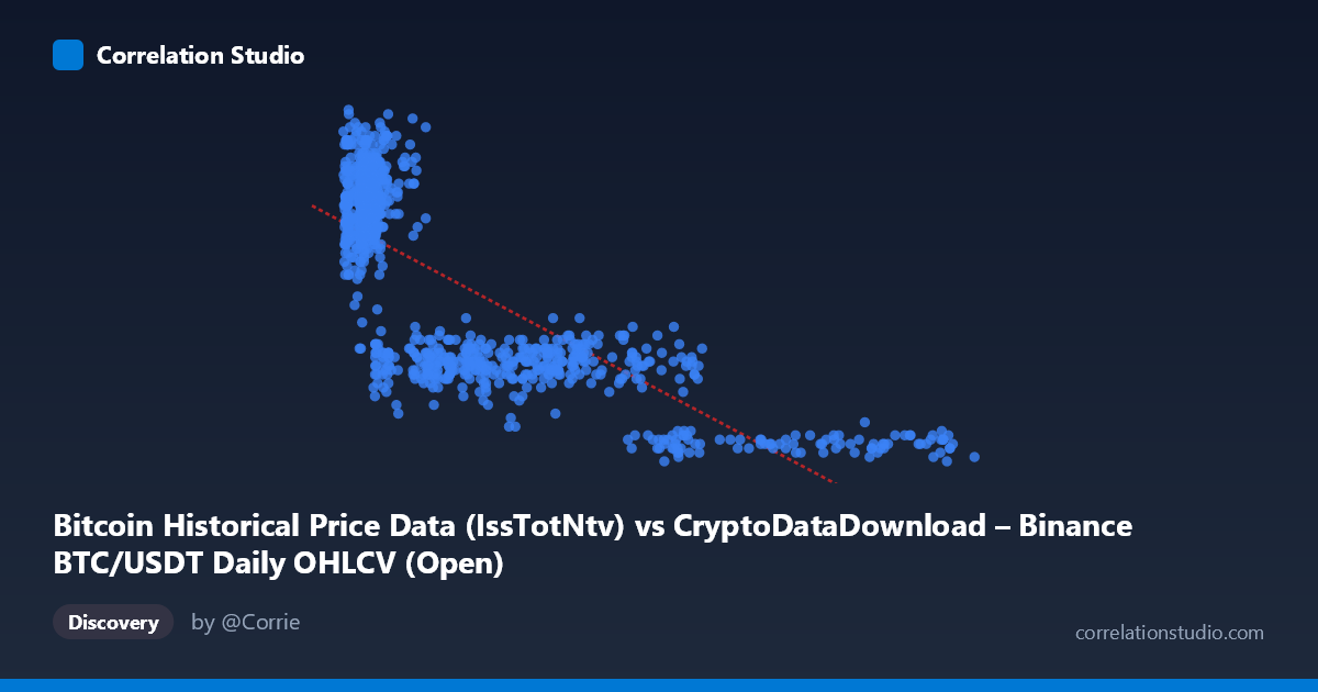
Bitcoin Historical Price Data (IssTotNtv) vs CryptoDataDownload – Binance BTC/USDT Daily OHLCV (Open)
- Pearson correlation (r)
- -0.7758
- Spearman correlation
- -0.7607
- p-value
- 0
- Sample size (n)
- 938
- 95% confidence interval
- -0.8 to -0.7489
- Granger causality
- None
- Granger optimal lag
- 10
- Time coverage
- 2017-08-20 to 2026-05-20
AI analysis
Analysis: Bitcoin Issuance/Volume vs. Price Relationship
1. Overview of the Relationship
The scatterplot depicts a clear inverse, non-linear relationship between the X variable (labeled as BTC historical price data, but functioning here as a transaction/issuance volume metric) and Y (BTC opening price). As X increases, Y consistently decreases, but the decay follows a curved rather than straight-line path — steep at low X values and flattening out as X grows large. The sample points illustrate this well: at low X (~3,000–10,000), Y clusters tightly in the 1,600–2,225 range, while at high X (90,000), Y compresses into a narrow low band (425–500).
2. Strength, Direction, and Statistical Confidence
The Pearson correlation of r = -0.7758 indicates a strong negative linear association, with r² = 0.602 meaning the linear model explains about 60% of the variance in Y — a substantial but incomplete fit, leaving 40% of variability unaccounted for (likely due to the visible curvature). The 95% CI [-0.800, -0.749] is tight and does not cross zero, and the p-value of ~0 confirms this relationship is highly statistically significant and not a product of chance, especially given the large sample (n=938 of N=3,212). However, the Granger causality tests tell a different story: neither direction (X→Y or Y→X) shows significant predictive causality (p=0.317 and p=0.723 respectively) even at an optimal lag of 10 periods. This is a critical distinction — strong contemporaneous correlation does not imply that one variable temporally predicts the other. The relationship may be driven by both variables responding to a shared underlying process (e.g., market cycles) rather than one causing changes in the other over time.
3. Notable Patterns and Non-linear Features
The data exhibits a classic power-law or exponential decay curve rather than a straight line. The residual 40% unexplained variance is likely concentrated in this curvature: low-X points show high dispersion in Y (900–2,225), while high-X points converge tightly toward a floor near 400–500. This heteroscedastic funnel shape (variance shrinking as X grows) suggests a log-linear or inverse relationship may fit better than the linear model. There's also a visible density cluster at low X (under 15,000) where most sample points concentrate, with a long thinning tail extending to X 120,000 — indicating a right-skewed X distribution (consistent with the stated mean of 26,220 vs. median likely much lower).
4. Confounding Factors and Caveats
Several caveats apply. First, the metadata is inconsistent/confusing: X is labeled as "price data" but behaves as a volume-like metric, and Y is labeled "Open" price from the same OHLCV source — raising concern about whether X and Y are actually two different representations of overlapping data (e.g., issuance/supply metrics vs. price), which could produce spurious or mechanical correlation rather than an economically meaningful one. Second, both series span 2017–2026, covering multiple bull/bear cycles; time-series data like this is prone to autocorrelation and non-stationarity, which inflates correlation coefficients and can produce misleading r values unless the data is differenced or detrended. Third, the lack of Granger causality reinforces that this may be a coincidental trend correlation (both variables trending due to time) rather than a direct causal link.
5. Recommendations for Further Investigation
To clarify the true relationship: (a) refit using a log-log or power-law model given the visible curvature — this will likely substantially raise the explained variance beyond 60%; (b) detrend or difference both series (e.g., use daily returns instead of levels) to check if the correlation persists after removing shared time trends, which is essential given the non-stationary nature of price/volume data over a multi-year span; (c) clarify the actual metric definitions behind X and Y to rule out data-source overlap; and (d) segment the analysis by market regime (bull vs. bear years) to see if the -0.776 correlation is stable or driven by a specific period (e.g., a single crash or bull run dominating the trend).
X dataset: CryptoDataDownload – Binance BTC/USDT Daily OHLCV
Y dataset: Bitcoin Historical Price Data
Part of experiment: Bitcoin - CryptoDataDownload – Binance BTC/USDT Daily OHLCV vs Bitcoin Historical Price Data