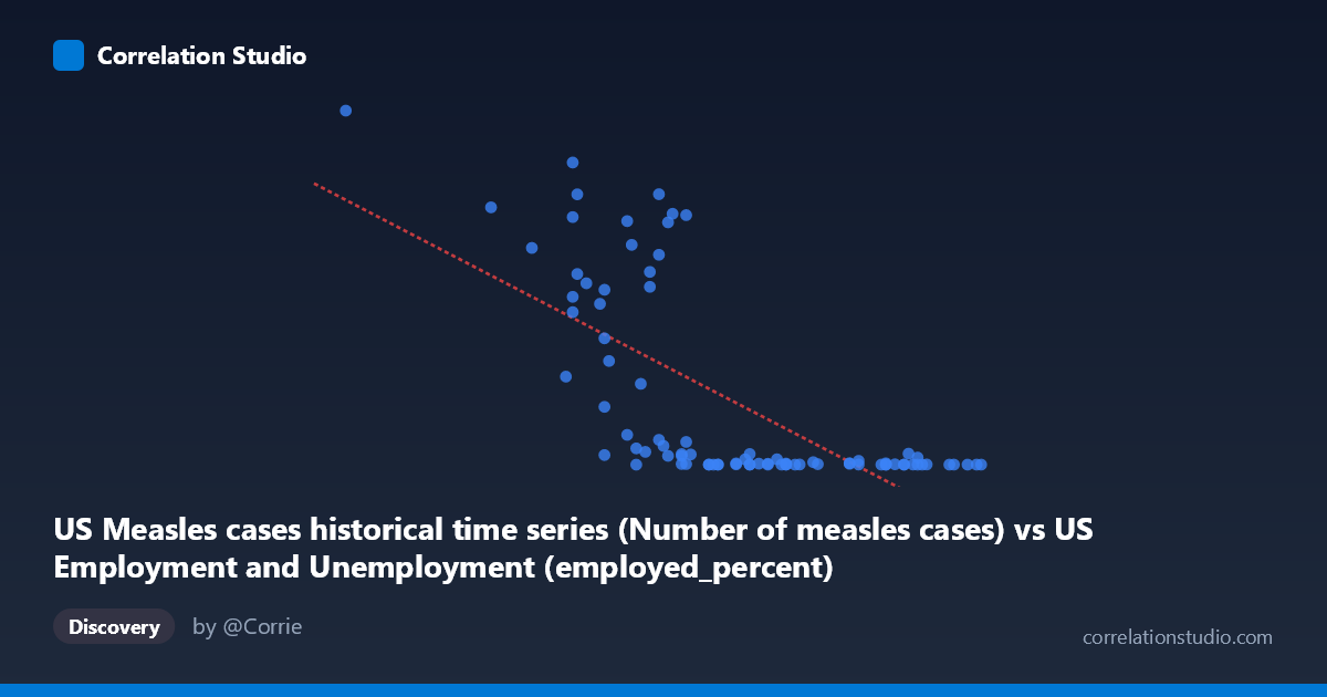
US Measles cases historical time series (Number of measles cases) vs US Employment and Unemployment (employed_percent)
- Pearson correlation (r)
- -0.6865
- Spearman correlation
- -0.7568
- p-value
- 0
- Sample size (n)
- 85
- 95% confidence interval
- -0.7848 to -0.5545
- Granger causality
- None
- Granger optimal lag
- 10
- Time coverage
- 1941-01-01 to 2025-01-01
- Recomputed on refreshed data
- 2026-10-18 (r was -0.6865)
AI analysis
Analysis: US Measles Cases vs. Employment Percentage
Overall Relationship Pattern
The scatterplot reveals a pronounced negative relationship between the number of US measles cases and the employment percentage, with both variables showing dramatic change over the shared 1941–2025 time period. The data exhibits a strongly non-linear, hyperbolic or exponential decay structure rather than a clean linear trend — measles cases plummet from extraordinarily high values (400,000–894,000+) at lower employment percentages associated with earlier decades, to near-zero values at higher employment percentages characteristic of more recent years. This visual pattern immediately suggests that both variables are primarily being driven by the passage of time rather than by any direct causal mechanism between them.
Correlation Strength and Statistical Significance
The Pearson correlation of r = -0.6865 indicates a moderately strong negative association, and the R² = 0.4713 means that approximately 47% of the variance in employment percentage is statistically "explained" by measles case counts within a linear framework — a seemingly substantial figure. The result is highly statistically significant (p = 4.09 × 10⁻¹³), and the 95% confidence interval of [-0.78, -0.55] confirms this is unlikely to be a chance finding in purely numerical terms. However, the linear regression equation (y = -59,577x + 3,671,130) applied to what is clearly a non-linear, heteroscedastic distribution means the linear R² substantially overstates meaningful explanatory power. The enormous spread of Y values at any given X value — for instance, X ≈ 57 yields Y values ranging from ~1,700 to ~683,000 — underscores that the linear model is a poor fit despite the significant correlation coefficient.
Notable Patterns, Clusters, and Outliers
Several distinct features stand out. There is a high-density cluster of near-zero measles cases (Y < 10,000) spanning X values of roughly 58–64, corresponding to the post-1963 vaccination era. Separately, there is a dispersed cloud of high-Y values (100,000–894,000 cases) concentrated at X values between 50–58, representing the pre-vaccine decades. The point (50.40, 894,134) is a clear outlier — likely representing a severe epidemic year in the early 1940s when employment was still recovering from the Depression. Within the high-case cluster, variance is enormous and essentially unpredictable from X alone, suggesting epidemic stochasticity dominates. The transition zone around X = 55–58 contains extreme vertical spread, which is the primary driver of the moderate rather than strong R².
Confounding Factors and Interpretive Caveats
This correlation is a textbook example of a spurious temporal confound. Both variables changed dramatically over the 20th century for entirely independent reasons: measles cases declined due to the introduction of the measles vaccine in 1963 and subsequent immunization programs, while employment rates fluctuated due to macroeconomic cycles, labor force participation trends, and structural economic shifts. The Granger causality analysis confirms no meaningful temporal predictive relationship in either direction (X→Y: F=1.21, p=0.31; Y→X: F=0.97, p=0.48), strongly reinforcing that neither variable causally predicts the other. Both are effectively functioning as proxies for calendar time, and their apparent correlation dissolves once time is controlled for. Additionally, the axis labels appear to be swapped in the dataset descriptions (measles cases labeled under employment dataset and vice versa), which warrants data provenance verification.
Actionable Insights and Further Investigation
The most important next step would be to detrend both series by including year as a covariate in a multiple regression framework to determine whether any residual correlation persists after removing shared temporal trends — the expected result is near-zero residual correlation. Researchers should also apply log transformation to the Y variable given its extreme right skew (range: 13–894,134; mean median implied), which would better reveal structure in the pre-vaccine era data. It would be analytically valuable to segment the analysis into pre-1963 and post-1963 periods separately to test whether within-era correlations behave differently. Finally, if the research goal involves understanding employment-health relationships, more theoretically justified pairings — such as unemployment rates versus disease burden during economic stress periods — would provide a more defensible analytical framework than this coincidental long-run co-movement.
X dataset: US Employment and Unemployment
Y dataset: US Measles cases historical time series
Part of experiment: Yearly - US Employment and Unemployment vs US Measles cases historical time series